In here, we discussed several examples of optimizations problems, mostly geometric optimization problems. In this note, we study business and economic optimization problems. Let us begin with the following example.

Example. Suppose that the price and demand for a particular luxury automobile are related by the demand equation $p+10x=200,000$, where $p$ is the price per car in dollars and $x$ is the number of cars that will be purchased at that price. What price should be charged per car if the total revenue is to be maximized?

Solution. Recall that the total revenue $R$ is given by $R=xp$, where $p$ is the price per item and $x$ is the number of items sold. In terms of $x$, the revenue is written as
$$R(x)=200,000x-10x^2$$
$R(x)=200,000-20x$ and set it equal to 0, we find the critical point $x=10,000$. Since $R^{\prime\prime}(x)=-20<0$, $R(10,000)=100,000,0000$, i.e. a billion dollars. We don’t actually calculus to see this. $R(x)$ is a quadratic function with negative leading coefficient, so it assumes as maximum at the $x$-coordinate of its vertex, $x=-\frac{b}{2a}=-\frac{200,000}{2\cdot 10}=10,000$. To answer the question, the price at which the total revenue $R$ is maximized is
$$p=-10(10,000)+200,000=100,000\ \mathrm{dollars}$$
As you might have noticed by now, it could have been shorter if we wrote $R$ in terms of the price $p$ since the question is about the price at which the revenue is maximized. In terms of $p$, $R$ is written as
$$R(p)=-\frac{p^2}{10}+20,000p$$
Either by solving $R'(p)=-\frac{p}{10}+20,000=0$ or by $p=-\frac{b}{2a}=\frac{20,000}{\frac{2}{10}}$, we find $p=\$ 100,000$.

Example. Suppose that the cost, in dollars, of producing $x$ hundred bicycles is given by $C(x)=x^2-2x+4900$. What is the minimum cost?

Solution. Either by solving $C'(x)=2x-2=0$ or by $x=-\frac{b}{2a}=-\frac{-2}{2\cdot 1}$, we find that $C(x)$ assumes the minimum at $x=1$, i.e. the cost of production is the minimum when 100 bicycles are produced. The minimum cost is $C(1)=4899$ dollars.

Example. In the preceding example, find the minimum average cost.

Solution. Recall that the average cost $\bar C(x)$ is given by $\bar C(x)=\frac{C(x)}{x}$, so we have
$$\bar C(x)=x-2+\frac{4900}{x}$$
Setting $C'(x)=1-\frac{4900}{x^2}$ equal to 0, we find $x=70$. Since $C^{\prime\prime}(x)=\frac{9800}{x^3}>0$ when $x=70$, $\bar C(70)=138$ (in dollars) is the minimum average cost.

Here is an interesting theorem from economics.

Theorem. The average cost is minimized at a level of production at which marginal cost equals average cost, i.e. when
$$C'(x)=\bar C(x)$$

Proof. Since $\bar C(x)=\frac{C(x)}{x}$, we obtain by the quotient rule
$$\bar C'(x)=\frac{xC'(x)-C(x)}{x^2}$$
Setting $\bar C'(x)=0$, we have
$$xC'(x)-C(x)=0,$$
that is
$$C'(x)=\frac{C(x)}{x}=\bar C(x)$$

The preceding example can be quickly answered using this Theorem. Setting $C'(x)=\bar C(x)$, we have
$$2x-2=x-2+\frac{4900}{x}$$
Simplifying this we obtain
$$x^2=4900$$
Hence, $x=70$ as we found earlier.

Example. The cost in dollars of producing $x$ stereos is given by $C(x)=70x+800$. The demand equation is $20p+x=18000$. (a) What level of production maximizes profit? (b) What is the price per stereo when profit is maximized? (c) What is the maximum profit?

Solution. From the demand equation, we obtain $p=-0.05x+900$. Recall that the profit function $P(x)$ is given by
\begin{align*} P(x)&=R(x)-C(x)\\ &=xp-C(x)\\ &=-0.05x^2+900x-(70x+800)\\ &=0.05x^2+830x-800 \end{align*}
Setting $P'(x)=-0.1 x+830$ equal to 0, we find the critical point $x=8300$. $P^{\prime\prime}(x)=-0.1<0$, so the profit has the maximum at $x=8300$.

(a) The level of production that maximizes profit is $x=8300$.

(b) The price per stereo at which profit is maximized is
$$p=-0.05(8300)+900=485\ \mathrm{dollars}$$

(c) The maximum profit is
$$P(8300)=-0.05(8300)^2+830(8300)-800=3,443,700\ \mathrm{dollars}$$

Here is another interesting theorem from economics.

Theorem. The profit is maximized when the marginal revenue equals the marginal cost, that is, when $R'(x)=C'(x)$.

Proof. Differentiating revenue function $P(x)=R(x)-C(x)$, we have
$$P'(x)=R'(x)-C'(x)$$
The critical point is obtained from $P'(x)=0$, i.e. when $R'(x)-C'(x)=0$ or $R'(x)=C'(x)$. That is, when the marginal revenue equals the marginal cost. This completes the proof.

The preceding example can be answered quickly using this theorem. Setting $R'(x)=C'(x)$, we have
$$-0.1x+900=70$$
or
$$x=8300$$

Example. A theater has 204 seats. The manager finds that he can fill all the seats if he charges \$4.00 per ticket. For each ten cents that he raises the ticket price he will sell three fewer seats. What ticket price should he charge to maximize the ticket revenue?

Solution. When the manager increases $n$ cents per ticket price, the number $x(n)$ of tickets sold is $x(n)=204-3n$ and the price $p(n)$ per ticket is $p(n)=4+0.1n$. Then the total revenue is given by
\begin{align*} R(n)&=x(n)p(n)\\ &=(204-3n)(4+0.1n)\\ &=-0.3n^2+8.4n+816 \end{align*}
Setting $R'(n)=-0.6n+8.4$ equal to 0, we find $n=14$. Since $R^{\prime\prime}(n)=-0.6<0$, the ticket revenue is maximized when $n=14$, i.e. when the ticket price is \$4.00+\$1.40=\$5.40.

Alternatively, one can easily find the demand equation which is linear in this case. The equation of line through two points $(204,4)$ and $(201,4.1)$ is given by
$$p=-\frac{1}{30}x+\frac{54}{5}$$
and so we obtain the revenue function
$$R(x)=-\frac{1}{30}x^2+\frac{54}{5}x$$
Setting $R'(x)=-\frac{x}{!5}+\frac{54}{5}$ equal to 0, we find $x=162$ and plugging this into the demand equation for $x$ gives $p=5.40$.

Let us consider a demand equation given as $x=D(p)$. If one were to consider $\frac{dx}{dp}$, the rate of change of demand with respect to price, often it would be convenient to have it as a dimensionless quantity, i.e. one that does not depend on particular units. For that we define a new quantity by dividing $\frac{dx}{dp}$ by $\frac{x}{p}$. The resulting ratio is called the elasticity of demand and is denoted by $\epsilon_D$.

Definition. The elasticity of demand $\epsilon_D$ is defined by
$$\epsilon_D=\frac{\frac{dx}{dp}}{\frac{x}{p}}=\frac{p}{x}\frac{dx}{dp}$$

In economics, demand decreases as price increases, so demand function is a decreasing function, i.e. $\frac{dx}{dp}<0$. Since both $x$ and $p$ are positive, the elasticity $\epsilon_D$ is always negative. The demand is said to be elastic if $|\epsilon_D|>1$, inelastic if $|\epsilon_D|<1$, and unitary if $|\epsilon_D|=1$.

Definition. The relative change of a function whose equation is $p=f(a)$ as $q$ changes from $q_1$ to $q_2$ is
$$\frac{f(q_2)-f(q_1)}{f(q_1)}$$
The percentage change is defined as
$$100\times\frac{f(q_2)-f(q_1)}{f(q_1)}$$

Example. (a) If the demand equation is $x=100-3p$ , find the elasticity of demand when $p=1$.

(b) Show that the elasticity equals the ratio of the relative change in demand to the relative change in price when $p$ changes from 1 to 2.

Solution. (a) $x=100-3p$, $\frac{dx}{dp}=-3$, and when $p=1$, $x=97$, so
$$\epsilon_D=\frac{p}{x}\frac{dx}{dp}=-\frac{3}{97}$$
Since $|\epsilon_D|<1$, the demand is inelastic.

(b) As $p$ changes from 1 to 2, the relative change in price is $\frac{2-1}{1}=1$. When $p$ changes from 1 to 2, $x$ changes from 97 to 94, so the relative change in demand is $-\frac{3}{97}$. Hence, the ration of the relative change in demand to the relative change in price is
$$\frac{-\frac{3}{97}}{1}=-\frac{3}{97}=\epsilon_D$$

Example. Given the demand equation $x=\sqrt{100-2p}$, find the elasticity of demand when $p=18$. Is the demand elastic or inelastic at $p=18$?

Solution. The elasticity $\epsilon_D$ at $p=18$ is
\begin{align*} \epsilon_D&=\frac{p}{x}\frac{dx}{dp}\\ &=\frac{18}{\sqrt{100-2(18)}}\left(-\frac{1}{\sqrt{100-2p}}\right)_{p=18}\\ &=\frac{18}{8}\left(-\frac{1}{8}\right)\\ &=-\frac{9}{32} \end{align*}
Since $|\epsilon_D|=\frac{9}{32}<1$, the demand at $p=18$ is inelastic.

Example. Show that when the revenue is maximized, $|\epsilon_D|=1$.

Solution. The total revenue is $R=xp$, so
\begin{align*} \frac{dR}{dp}&=\frac{dx}{dp}p+x\\ &=x\left(1+\frac{p}{x}\frac{dx}{dp}\right)\\ &=x(1+\epsilon_D) \end{align*}
Since $x>0$, $\frac{dR}{dp}=0$ if and only if $\epsilon_D=-1$. If $\epsilon_D<-1$, then $|\epsilon_D|>1$ i.e. the demand is elastic, and $\frac{dR}{dp}<0$ (the revenue is decreasing). If $-1<\epsilon_D<0$, then $|\epsilon_D|<1$ i.e. the demand is inelastic, and $\frac{dR}{dp}>0$ (the revenue is increasing). So, the revenue is maximized when $|\epsilon_D|=1$.

When demand is a function of price, the elasticity can be written as
$$\epsilon_D=\frac{\frac{p}{x}}{\frac{dp}{dx}}$$

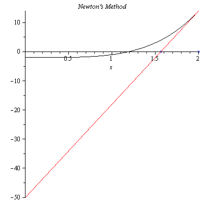
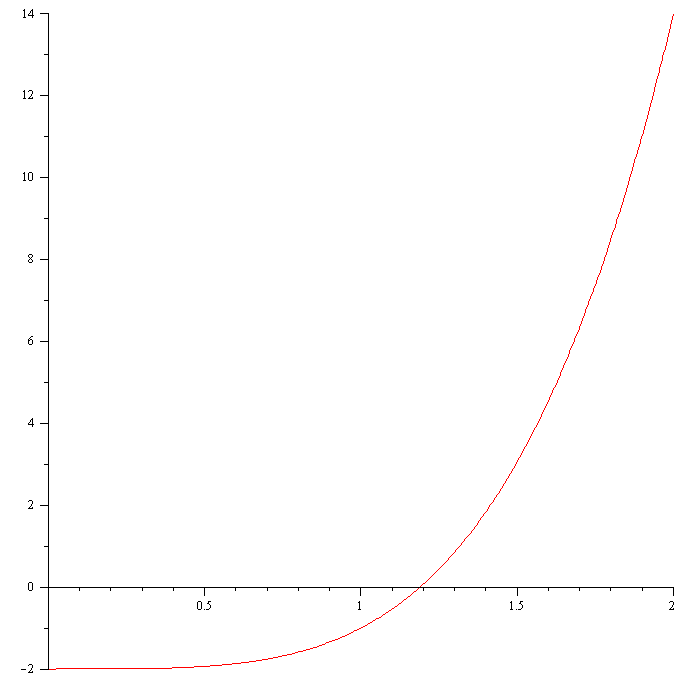
Quadratic equations can be easily solved using the quadratic formula. For cubic and quartic equations there are also formula for solutions, but they are pretty complicated. For polynomials of higher-order degree of 5 or higher there are no such formulas for roots. Newton’s Method allows us to find an approximate solution to such equations. I will use a simple example to explain how it works and then formulate Newton’s method in general. Let us consider the function $f(x)=x^4-2$. Newton’s method begins with by guessing the first solution. In order for Newton’s method to work, one needs to come up with the first guess close enough to the actual solution, otherwise Newton’s method may return an undesirable result. (I will show you an example of such case later on.) We can come up with a reasonable first guess say $x_0$ using the graph of the function.

From the graph, we choose $x_0=2$. Of course, one can choose even a closer point, for example $x_0=1.5$. The tangent line to the graph of $f(x)$ at $x_0=2$ is
$$y-f(x_0)=f'(x_0)(x-x_0)$$
Setting $y=0$, we find the $x$-intercept $x_1$
$$x_1=x_0-\frac{f(x_0)}{f'(x_0)}=1.562500000$$

In Figure 2, we see that $x_1$ is closer to the actual solution than $x_0$. This time we find the $x$-intercept $x_2$ of the tangent line to the graph of $f(x)$ at $x_1=1.562500000$.
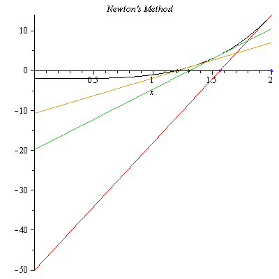
$$x_2=x_1-\frac{f(x_1)}{f'(x_1)}=1.302947000$$

In Figure 3, we see that $x_2$ is closer to the actual solution than $x_1$. Similarly, we can find the next approximate solution $x_3=1.203252569$ which is closer to the actual solution than $x_2$ as shown in Figure 3.

Continuing this process, the 6th approximate solution is given by $x_6=1.189207115$ which is correct to 9 decimal places. The exact solution is $\root 4\of{2}=1.189207115002721$.

In general, Newton’s Method is given by
\begin{align*}x_0&=\mbox{initial approximate}\\x_{n+1}&=x_n-\frac{f(x_n)}{f'(x_n)}\end{align*}
for $n=0,1,2,\cdots$. Here, the assumption is that $f'(x_n)\ne 0$ for $n=0,1,2,\cdots$.

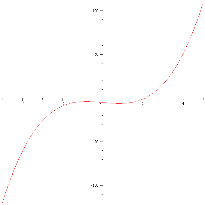
Earlier, I mentioned that if we don’t choose the initial approximate $x_0$ close enough to the actual solution, Newton’s method may return an undesirable result. Let me show you an example. Let us consider the function $f(x)=x^3-2x-5$. Figure 4 shows its graph.

If we choose $x_0=-4$ and run Newton’s method, we obtain the following approximates.

                  X[1] = -2.673913043
                  X[2] = -1.708838801
                  X[3] = -0.7366532045
                  X[4] = -11.29086856
                  X[5] = -7.553673519
                  X[6] = -5.065760748
                  X[7] = -3.400569565
                  X[8] = -2.252794796
                  X[9] = -1.350919123
                 X[10] = 0.01991182580
                 X[11] = -2.501495587
                 X[12] = -1.568413258
                 X[13] = -0.5049189040

As we can see, the numbers do not not appear to be converging to somewhere which indicates that Newton’s method is not working well for this case. In certain cases when we choose $x_0$ too far from the actual solution, we may end up getting $f'(x_n)=0$ for some $n$ in which case Newton’s method fails. For $x_0=4$, we obtain

                   X[1] = 2.891304348
                   X[2] = 2.311222795
                   X[3] = 2.117035157
                   X[4] = 2.094830999
                   X[5] = 2.094551526

The fifth approximate $x_5=2.094551526$ is correct to 6 decimal places.

Newton’s method is not suitable to be carried out by hand. An open source computer algebra system Maxima has a built-in package mnewton for Newton’s method. If you want to install Maxima on your computer, you can find an instruction here. Let us redo the above example using mnewton with initial approximate $x_0=4$.

(%i1) load(“mnewton”)$
(%i2) mnewton([x^3-2*x-5], [x], [4]);
(%o2) [[x = 2.094551481542326]]

What I find interesting about mnewton is that even if you use an initial approximate that didn’t work out for the standard Newton’s method such as $x_0=-4$ in the above example, it instantly returns the answer. (Try it yourself.)

Newton’s method can be used to calculate internal rate of return (IRR) in finance. It is the discount rate at which net present value (NPV) is equal to zero. NPV is the sum of the present values of all cash flows, or alternatively, NPV can be defined as the difference between the present value of the benefits (cash inflows) and the present value of the costs (cash outflows). Here is an example.

Example. If we invest \$100 today and receive \$110 in one year, then NPV can be expressed as
$$\mathrm{NPV}=-100+\frac{110}{1+\mathrm{IRR}}$$
Setting $\mathrm{NPV}=0$, we have
$$\mathrm{IRR}=\frac{110}{100}-1=0.1=10\%$$
If we have multiple future cash inflows \$90, \$50, and \$30 at the end of each year for the next three years, NPV is given by
$$\mathrm{NPV}=-100+\frac{90}{1+\mathrm{IRR}}+\frac{50}{(1+\mathrm{IRR})^2}+\frac{30}{(1+\mathrm{IRR})^3}$$
Setting $\mathrm{NPV}=0$, we obtain a cubic equation
$$100x^3-90x^2-50x-30=0$$
where $x=1+\mathrm{IRR}$. Using Newton’s method, we find $x=1.41$, so $\mathrm{IRR}=0.41=41\%$.

(%i1) load(“mnewton”)$
(%i2) mnewton([100x^3-90x^2-50*x-30], [x], [1]);
(%o2) [[x = 1.406937359155343]]

Update: I wrote a simple Maple script that runs Newton’s method. If you have Maplesoft, you are more than welcome to download the Maple worksheet here and use it.

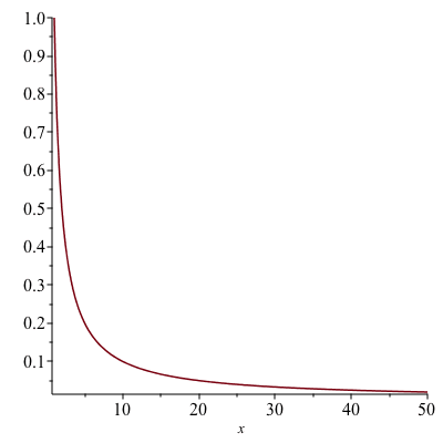
Consider the curve $y=\frac{1}{x}$, $1\leq x<\infty$.

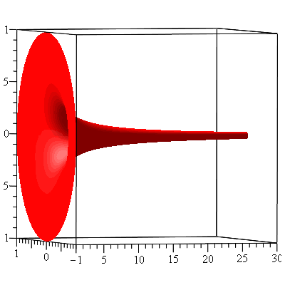
Gabriel’s horn is the surface that is obtained by rotating the above curve about the x-axis.

What’s interesting about this Gabriel’s horn is that its surface area is infinite while the volume of its interior is finite. Let us first calculate the volume. Using the disk method, the volume is given by \begin{align*}V&=\pi\int_1^\infty\left(\frac{1}{x}\right)^2dx\\&=\pi\lim_{a\to\infty}\int_1^a\frac{1}{x^2}dx\\&=\pi\lim_{a\to\infty}\left[-\frac{1}{x}\right]_1^a\\&=\pi\lim_{a\to\infty}\left[1-\frac{1}{a}\right]\\&=\pi\end{align*}Its surface area is obtained by calculating the integral \begin{align*}A&=2\pi\int_1^\infty\frac{1}{x}\sqrt{1+\left(-\frac{1}{x^2}\right)^2}dx\\&=2\pi\lim_{a\to\infty}\int_1^a\frac{1}{x}\sqrt{1+\frac{1}{x^4}}dx\end{align*} We don’t actually have to evaluate this integral to see the area is infinite. Since $\sqrt{1+\frac{1}{x^4}}>1$, $$\int_1^a\frac{1}{x}\sqrt{1+\frac{1}{x^4}}dx\geq \int_1^a\frac{1}{x}dx=\ln a$$ Hence, $A=\infty$. The integral $\int \frac{1}{x}\sqrt{1+\frac{1}{x^4}}dx$ can be evaluated exactly. Using first the substitution $u=x^2$ and then the trigonometric substitution $u=\tan\theta$, \begin{align*}\int\frac{1}{x}\sqrt{1+\frac{1}{x^4}}dx&=\frac{1}{2}\int\frac{\sqrt{1+u^2}}{u^2}du\\&=\frac{1}{2}\int\frac{\sec^2\theta\sec\theta}{\tan^2\theta}d\theta\\&=\frac{1}{2}\int\frac{(1+\tan^2\theta)\sec\theta}{\tan^2\theta}d\theta\\&=\frac{1}{2}\left[\int\cot^2\theta\sec\theta d\theta+\int\sec\theta d\theta\right]\\&=\frac{1}{2}\left[\int\frac{\cos\theta}{\sin^2\theta}d\theta+\int\sec\theta d\theta\right]\\&=\frac{1}{2}\left[-\csc\theta+\ln|\sec\theta+\tan\theta|\right]\\&=\frac{1}{2}\left[-\frac{\sqrt{x^4+1}}{x^2}+\ln(\sqrt{x^4+1}+x^2)\right]\end{align*}

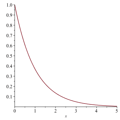
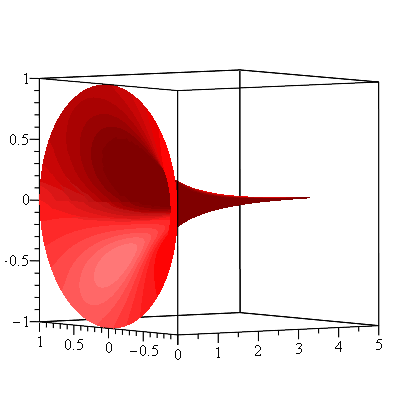
Another horn-shaped surface can be obtained by rotating the curve $y=e^{-x}$, $0\leq x<\infty$:

The volume of the interior is finite and \begin{align*}V&=\pi\int_0^\infty e^{-2x}dx\\&=\pi\lim_{a\to\infty}\int_0^\infty e^{-2x}dx\\&=-\frac{\pi}{2}\lim_{a\to\infty}[e^{-2x}]_0^a\\&=\frac{\pi}{2}\end{align*} Unlike Gabriel’s horn, the surface area is also finite. To see that, it is given by the improper integral \begin{align*}A&=\int_0^\infty 2\pi e^{-x}\sqrt{1+(-e^{-x})^2}dx\\&=2\pi\lim_{a\to\infty}\int_0^a e^{-x}\sqrt{1+e^{-2x}}dx\end{align*} Using the substitution $u=e^{-x}$ and then the trigonometric substitution $u=\tan\theta$ the integral $\int e^{-x}\sqrt{1+e^{-2x}}dx$ is evaluated to be \begin{align*}\int e^{-x}\sqrt{1+e^{-2x}}dx&=-\int\sqrt{1+u^2}du\\&=-\int\sec^3\theta d\theta\\&=-\frac{1}{2}[\sec\theta\tan\theta+\ln|\sec\theta+\tan\theta|]\\&=-\frac{1}{2}[u\sqrt{1+u^2}+\ln|\sqrt{u^2+1}+u|]\\&=-\frac{1}{2}[e^{-x}\sqrt{e^{-2x}+1}+\ln(\sqrt{e^{-2x}+1}+e^{-x})]\end{align*} (For the details on how to evaluate the integral $\int\sec^3\theta d\theta$, see here.) Hence, $A$ is computed to be $\pi[\sqrt{2}+\ln(\sqrt{2}+1)]$.

Update: Instead of doing substitutions twice as seen above, one can use a single substitution $e^{-x}=\tan\theta$. The area then turns into the integral $$A=2\pi\int_0^{\frac{\pi}{4}}\sec^3\theta d\theta$$

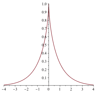
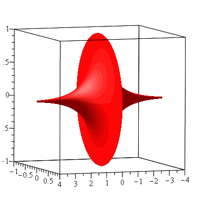
There is a particularly interesting horn-shaped surface (actually a shape of two identical horns put together as shown in the figure below) although it has both a finite volume and a finite surface area. It is called a pseudosphere. A pseudosphere is a surface with constant negative Gaussian curvature. The pseudosphere of radius 1 is obtained by revolving the tractrix $$t\mapsto (t-\tanh t,\mathrm{sech}\ t),\ -\infty<t<\infty$$ about its asymptote (the $x$-axis).

The resulting surface of revolution, the pseudosphere of radius 1, is seen in the following figure.

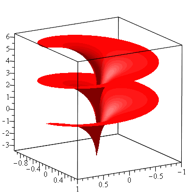
The volume of the interior of the pseudosphere is \begin{align*}V&=\pi\int_{-\infty}^\infty y^2dx\\&=2\pi\int_0^\infty y^2dx\\&=2\pi\int_0^\infty\mathrm{sech}^2\ t (1-\mathrm{sech}^2\ t)dt\\&=2\pi\int_0^\infty \mathrm{sech}^2\ t\tanh^2 tdt\\&=2\pi\int_0^1 u^2du\ (u=\tanh t)\\&=2\pi\left[\frac{u^3}{3}\right]_0^1\\&=\frac{2\pi}{3}\end{align*} The area of the pseudosphere is \begin{align*}A&=\int_{-\infty}^\infty 2\pi y ds\\&=2\int_0^\infty 2\pi y\sqrt{\left(\frac{dx}{dt}\right)^2+\left(\frac{dy}{dt}\right)^2}dt\\&=4\pi\int_0^\infty\mathrm{sech}\ t\sqrt{(1-\mathrm{sech}^2\ t)^2+(-\mathrm{sech}\ t\tanh t)^2}dt\\&=4\pi\int_0^\infty\mathrm{sech}\ t\sqrt{\tanh^4 t+\mathrm{sech}^2 t\tanh^2 t}dt\\&=4\pi\int_0^\infty\mathrm{sech}\ t\tanh t dt\\&=4\pi\int_0^\infty\frac{\sinh t}{\cosh^2 t}dt\\&=4\pi\int_1^\infty\frac{1}{u^2}du\ (u=\cosh t)\\&=4\pi\end{align*} Notice that its volume is half of the volume of the unit sphere and its area is the same as the area of the unit sphere. Such volume and area relationships are still true for the pseudosphere of radius $r$, i.e. the volume and the area of the pseudosphere of radius $r$ are, respectively, $\frac{2}{3}\pi r^3$ and $4\pi r^2$ (we do not discuss it here, but the radius of a pseudosphere is defined to be the radius of its equator) as noted by the Dutch physicist Christiaan Huygens. The Gaussian curvature of a regular surface can be computed by the Gauss’ formula. The pseudosphere of radius 1 as a parametric surface is represented by the equation $$\varphi(t,s)=(t-\tanh t,\mathrm{sech}\ t\cos s,\mathrm{sech}\ t\sin s)$$ As seen in the figure above, the pseudosphere is not regular along the equator (at $t=0$). It has a constant negative Gaussian curvature $K=-1$ anywhere else. A common misunderstanding (usually by non-mathematicians) is that a surface with constant negative Gaussian curvature is a hyperbolic surface. In order for a surface to be hyperbolic, in addition to having a constant negative curvature, it is required to be complete and regular, so the pseudosphere is not hyperbolic although it was introduced by Eugenio Beltrami as a model of hyperbolic geometry. In fact, Hilbert’s theorem states that there exist no complete regular surface of constant negative Gaussian curvature immersed in $\mathbb{R}^3$. This means that one cannot obtain a model of two-dimensional hyperbolic geometry in $\mathbb{R}^3$. However, one can obtain a model of two-dimensional hyperbolic geoemtry in $\mathbb{R^{2+1}}$, a 3-dimensional Minkowski space-time. There is another interesting surface with constant negative Gaussian curvature called Dini’s surface. It is described by the parametric equations \begin{align*}x&=a\cos u\sin v\\y&=a\sin u\sin v\\z&=a\left(\cos v+\ln\tan\frac{v}{2}\right)+bu\end{align*}

The Gaussian curvature of Dini’s surface is computed to be $K=-\frac{1}{a^2+b^2}$.

Related rates problems often involve (context-wise) real-life applications of the chain rule/implicit differentiation. Here are some of the examples that are commonly seen in calculus textbooks.

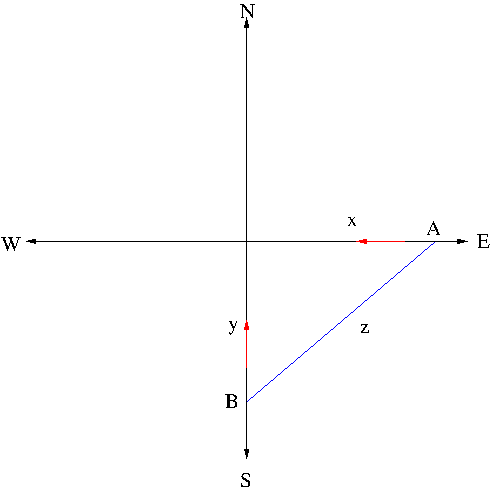
Example. Car A is traveling west at 50mi/h and car B is traveling north at 60mi/h. Both are headed for the intersection of the two roads. At what rate are the cars approaching each other when car A is 0.3 mi and car B is 0.4 mi from the intersection?

Solution.

Denote by $x$ and $y$ the distances from the intersection to car A and to car B, respectively. Then we have $\frac{dx}{dt}=-50$mi/h and $\frac{dy}{dt}=-60$mi/h. Let us denote $z$ the distance between $A$ and $B$. Then by Pythagorean law we have $$z^2=x^2+y^2$$ Differentiating this with respect to $t$, we obtain $$z\frac{dz}{dt}=x\frac{dx}{dt}+y\frac{dy}{dt}$$ and thus \begin{align*}\frac{dz}{dt}&=\frac{1}{z}\left[x\frac{dx}{dt}+y\frac{dy}{dt}\right]\\&=\frac{1}{0.5}[0.3(-50)+0.4(-60)]=-78\mathrm{mi/h}\end{align*}

Example. Air is being pumped into a spherical balloon so that its volume increases at a rate of $100\mathrm{cm}^3/\mathrm{s}$. How fast is the radius of the balloon increasing when the diameter is 50 cm?

Solution. Let $V$ and $r$ denote the volume and the radius of the spherical balloon. Then $V=\frac{4}{3}\pi r^3$. Differentiating this with respect to $t$, we obtain $$\frac{dV}{dt}=4\pi r^2\frac{dr}{dt}$$ So, \begin{align*}\frac{dr}{dt}&=\frac{1}{4\pi r^2}\frac{dV}{dt}\\&=\frac{1}{4\pi(25)^2}100\\&=\frac{1}{25\pi}\mathrm{cm/s}\end{align*}

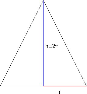
Example. Gravel is being dumped from a conveyor belt at a rate of $30 \mathrm{ft}^3/\mathrm{min}$ and its coarseness is such that it forms a pile in the shape of a cone whose base diameter and height are the same. How fast is the height of the pile increasing when the pile is 10 ft high?

Solution. The cross section of the gravel pile is shown in the figure below.

The amount of gravel dumped is the same as the volume of the cone. Let us denote the volume by $V$, its base radius by $r$, and its height by $h$. Then $V=\frac{1}{3}\pi r^2h$. Since $h=2r$, $V$ can be written as $$V=\frac{1}{12}\pi h^3$$ Differentiating this with respect to $t$, we obtain $$\frac{dV}{dt}=\frac{1}{4}\pi h^2\frac{dh}{dt}$$ So, we have \begin{align*}\frac{dh}{dt}&=\frac{4}{\pi h^2}\frac{dV}{dt}\\&=\frac{4}{\pi(10)^2}(30)=\frac{1.2}{\pi}\mathrm{ft/min}\approx 0.38\mathrm{ft/min}\end{align*}

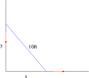
Example. A ladder 10 ft long rests against a vertical wall. If the bottom of the ladder slides away from the wall at a rate of 1 ft/s, how fast is the top of the ladder sliding down the wall when the bottom of the ladder is 6 ft from the wall?

Solution.

Let us denote by $x$ and $y$ the distance from the wall to the bottom of the ladder and the distance from the top of the ladder to the floor, respectively. By Pythagorean law, we have $x^2+y^2=100$. Differentiating this with respect to $t$, we obtain $$x\frac{dx}{dt}+y\frac{dy}{dt}=0$$ Hence, we have \begin{align*}\frac{dy}{dt}&=-\frac{x}{y}\frac{dx}{dt}\\&=-\frac{6}{8}(1)=-\frac{3}{4}\mathrm{ft/s}\end{align*}

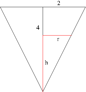
Example. A water tank has the shape of an inverted circular cone with base radius 2m and heigh 4 m. If water is being pumped into the tank at a rate of $2 \mathrm{m}^3/\mathrm{min}$, find the rate at which the water level is rising when the water is 3 m deep.

Solution. The cross section of the water tank is shown in the figure below.

The amount of water $V$ when the water level is $h$ and the surface radius is $r$ is $V=\frac{1}{3}\pi r^2h$. From the above figure we have the following ratio holds $$\frac{2}{4}=\frac{r}{h}$$ i.e. $r=\frac{h}{2}$. SO $V$ can be written as $$V=\frac{1}{12}\pi h^3$$ Differentiating this with respect to $t$, we obtain $$\frac{dV}{dt}=\frac{1}{4}\pi h^2\frac{dh}{dt}$$ Hence, \begin{align*}\frac{dh}{dt}&=\frac{4}{\pi h^2}\frac{dV}{dt}\\&=\frac{4}{\pi(3)^2}(2)\\&=\frac{8}{9\pi}\mathrm{m/min}\approx 0.28\mathrm{m/min}\end{align*}

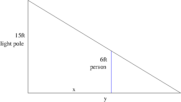
Example. A street light is at the top of a 15 feet tall pole. A 6 feet tall woman walks away from the pole with a speed of 5 ft/sec along a straight path. How fast is the tip of her shadow moving when she is 45 feet from the base of the pole?

Solution. Let $x$ be the distance from the light pole to the woman and $y$ be the distance from the light pole to the tip of her shadow as shown in the figure below.

By similar triangles, we have $\frac{15}{y}=\frac{6}{y-x}$. Solving this equation for $y$, we obtain $y=\frac{5}{3}x$. Differentiating this with respect to $t$, we find how fast the tip of her shadow is moving: $$\frac{dy}{dt}=\frac{5}{3}\frac{dx}{dt}=\frac{25}{3}\mathrm{ft/s}$$ As seen regardless of how far the woman is from the pole, the speed of the tip is constant.

Example. The fish population, $N$, in a small pond depends on the amount of algae, $a$ (measured in pounds), in it. The equation modeling the fish population is given by $N=(3a^2-20a+26)^4$. If the amount of algae is increasing at a rate of 2 lb/week, at what rate is the fish population changing when the pond contains 5 lb of algae?

Solution. By the chain rule, we obtain \begin{align*}\frac{dN}{dt}&=4(3a^2-20a+26)^3\left(6a\frac{da}{dt}-20\frac{da}{dt}\right)\\&=4(3a^2-20a+26)^3(6a-20)\frac{da}{dt}\end{align*} $\frac{da}{dt}=2$lb/week, so when $a=5$lb, $\frac{dN}{dt}$ is $$\frac{dN}{dt}=4(3(5)^2-20(5)+26)^3(6(5)-20)(2)=-80\ \mathrm{lb/week}$$ What this means is that the fish population is decreasing by 80 lb/week at the instant when the pond contains 5 lb of algae.

Example. The retail price per gallon of gasoline is increasing at \$0.02 per week. The demand equation is given by $$10p-\sqrt{356-x^2}=0$$ where $p$ is the price per gallon (in dollars), when $x$ million gallons are demanded. At what rate is the revenue changing when 10 million gallons are demanded?

Solution. The total revenue $R$ is given by the equation $$R=xp$$ Differentiating this equation with respect to $t$, we obtain $$\frac{dR}{dt}=\frac{dx}{dt}p+x\frac{dp}{dt}$$ The only quantity we don’t have to calculate $\frac{dR}{dt}$ is $\frac{dx}{dt}$. To find it, let us differentiate the demand function with respect to $x$. By the chain rule, we obtain $$10\frac{dp}{dt}+\frac{x}{\sqrt{351-x^2}}\frac{dx}{dt}=0$$ When $x=10$ million gallons, with $\frac{dp}{dt}=0.02$, we find from this equation that $$\frac{dx}{dt}=-0.02\sqrt{256}=-0.02\cdot 16= -0.32\ \mbox{million gallons/week}$$ When $x=10$, from the demand function, we find $p$ as $$p=\frac{\sqrt{256}}{10}=\frac{16}{10}=1.6$$ Therefore, the rate of change of revenue when 10 million gallons of gasoline is demanded is $$\frac{dR}{dt}=-0.32(1.6)+10(0.02)=-0.312$$ What this means is that the revenue is decreasing by about 0.31 million dollars per week when the price increases 0.02 dollars per week (consequently the demand decreases by 0.32 million gallons per week as we saw earlier).

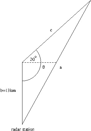
Example. A plane flying with a constant speed of 29 km/min passes over a ground radar station at an altitude of 13 km and climbs at an angle of 20 degrees. At what rate is the distance from the plane to the radar station increasing 3 minutes later?

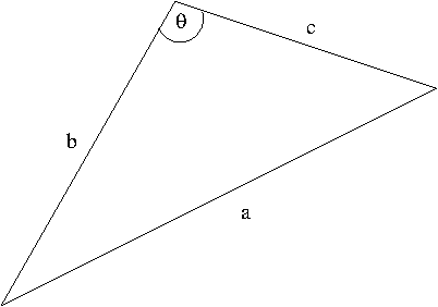
Solution. First, take a look at the following picture

The law of cosine says that the sides $a$, $b$, $c$ and the angle $\theta$ are related by $$a^2=b^2+c^2-2bc\cos\theta$$

The question above can be pictorially represented as the following sketch

Using the law of cosine with $b=13$ km, we have $$a^2=13^2+c^2-2\cdot 13\cdot c\cdot\cos\left(\frac{11}{18}\pi\right)$$ Here, the angle $\theta$ is given by $\theta=90^\circ+20^\circ=110^\circ=\frac{11}{18}\pi$$ (Note: for this question, you can use degree instead of radian but in that case make sure that your calculator is set to use degree angle measurement.) Since we are to find $\frac{da}{dt}$, differentiate the above equation with respect to $t$: $$2a\frac{da}{dt}=2c\frac{dc}{dt}-2\cdot 13\frac{dc}{dt}\cos\left(\frac{11}{18}\pi\right)$$ Since the airplane is flying along the side $c$ at the constant speed 29 km/min, it would have traveled $c=29\cdot 3=87$ km in three minutes. Thus, $$a=\sqrt{13^2+87^2-2\cdot 13\cdot 87\cos\left(\frac{11}{18}\pi\right)}=92.2586$$ and hence $\frac{da}{dt}$ in three minutes is \begin{align*}\frac{da}{dt}&=\frac{c}{a}\frac{dc}{dt}-\frac{13}{a}\frac{dc}{dt}\cos\left(\frac{11}{18}\pi\right)\\&=\frac{1}{a}\frac{dc}{dt}\left(c-13\cos\left(\frac{11}{18}\pi\right)\right)\\&=\frac{1}{92.2586}29\left(87-13\cos\left(\frac{11}{18}\pi\right)\right)\\&=28.7447\ \mathrm{km/min}\end{align*}

We have already discussed the length of a plane curve represented by the parametric equation ${\bf r}(t)=(x(t),y(t))$, $a\leq t\leq b$ here. The same goes for a space curve. Namely, if ${\bf r}(t)=(x(t),y(t),z(t))$, $a\leq t\leq b$, then its arc length $L$ is given by \begin{equation}\begin{aligned}L&=\int_a^b|{\bf r}'(t)|dt\\&=\int_a^b\sqrt{\left(\frac{dx}{dt}\right)^2+\left(\frac{dy}{dt}\right)^2+\left(\frac{dz}{dt}\right)^2}dt\end{aligned}\label{eq:spacearclength}\end{equation}

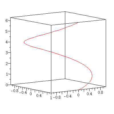
Example. Find the length of the arc of the circular helix $${\bf r}(t)=\cos t{\bf i}+\sin t{\bf j}+t{\bf k}$$ from the point $(1,0,0)$ to the point $(1,0,2\pi)$.

Solution. ${\bf r}'(t)=-\sin t{\bf i}+\cos t{\bf j}+{\bf k}$ so we have $$|{\bf r}'(t)|=\sqrt{(-\sin t)^2+(\cos t)^2+1^2}=\sqrt{2}$$ The arc is going from $(1,0,0)$ to $(1,0,2\pi)$ and the $z$-component of ${\bf r}(t)$ is $t$, so $0\leq t\leq 2\pi$. Now, using \eqref{eq:spacearclength}, we obtain $$L=\int_0^{2\pi}|{\bf r}'(t)|dt=\int_0^{2\pi}\sqrt{2}dt=2\sqrt{2}\pi$$ Figure 1 shows the circular helix from $t=0$ to $t=2\pi$.

Given a curve ${\bf r}(t)$, $a\leq t\leq b$, sometimes we need to reparametrize it by another parameter $s$ for various reasons. Imagine that the curve represents the path of a particle moving in space. A reparametrization does not change the path of the particle (hence nor the distance it traveled) but it changes the particle’s speed! To see this, let $t=t(s)$, $\alpha\leq s\leq\beta$, $a=t(\alpha)$, $b=t(\beta)$ be an increasing and differentiable function. Since $t=t(s)$ is one-to-one and onto, ${\bf r}(t)$ and ${\bf r}(t(s))$, its reparametrization by the parameter $s$, represent the same path. By the chain rule, \begin{equation}\label{eq:reparametrization}\frac{d}{ds}{\bf r}(t(s))=\frac{d}{dt}{\bf r}(t)\frac{dt}{ds}\end{equation} Thus we see that the speed of the reparametrization $\left|{\bf r}(t(s))\right|$ differs from that of ${\bf r}(t)$ by a factor of $\left|\frac{dt}{ds}\right|=\frac{dt}{ds}$ (since $\frac{dt}{ds}>0$). However, the arc length of the reparametrization is \begin{align*}\int_{\alpha}^{\beta}\left|\frac{d}{ds}{\bf r}(t(s))\right|ds&=\int_{\alpha}^{\beta}\left|\frac{d}{dt}{\bf r}(t)\right|\frac{dt}{ds}ds\\&=\int_a^b\left|\frac{d}{dt}{\bf r}(t)\right|dt=L\end{align*} That is, no change of the distance.

There is a particular reparametrization we are interested. To discuss that, suppose ${\bf r}(t)$, $a\leq t\leq b$ be a differentiable curve in space such that ${\bf r}'(t)\ne 0$ for all $t$. Such a curve is said to be regular or smooth. Let us now define the arc length function \begin{equation}\label{eq:arclengthfunction}s(t)=\int_a^t|{\bf r}'(u)|du\end{equation} By the Fundamental Theorem of Calculus, we have \begin{equation}\label{eq:arclengthfunction2}\frac{ds}{dt}=|{\bf r}'(t)|>0\end{equation} and so the arc length function $s=s(t)$ is increasing. This means that $s(t)$ is one-to-one and onto, so it is invertible. It’s inverse function can be written as $t=t(s)$ and ${\bf r}(t(s))$ is called the reparamerization by arc length. The reason we are interested in this particular reparametrization is that it results in the unit speed: From \eqref{eq:reparametrization} and \eqref{eq:arclengthfunction2}, $$\left|\frac{d}{ds}{\bf r}(t(s))\right|=|{\bf r}'(t)|\left|\frac{dt}{ds}\right|=|{\bf r}'(t)|\frac{1}{|{\bf r}'(t)|}=1$$ So it is also called the unit-speed reparametrization. The reparametrization by arc length plays an important role in defining the curvature of a curve. This will be discussed elsewhere.

Example. Reparametrize the helix ${\bf r}(t)=\cos t{\bf i}+\sin t{\bf j}+t{\bf k}$ by arc length measured from $(1,0,0)$in the direction of increasing $t$.

Solution. The initial point $(1,0,0)$ corresponds to $t=0$. From the previous example, we know that the helix has the constant speed $|{\bf r}'(t)|=\sqrt{2}$. Thus, $$s(t)=\int_0^t|{\bf r}'(u)|du=\sqrt{2}t$$ Hence, we obtain $t=\frac{s}{\sqrt{2}}$. The reparametrization is then given by $${\bf r}(t(s))=\cos\left(\frac{s}{\sqrt{2}}\right){\bf i}+\sin\left(\frac{s}{\sqrt{2}}\right){\bf j}+\frac{s}{\sqrt{2}}{\bf k}$$

Examples in this note have been taken from [1].

References.

[1] Calculus, Early Transcendentals, James Stewart, 6th Edition, Thompson Brooks/Cole