Category Archives: General Relativity

Black Hole 1: Schwarzschild Black Hole

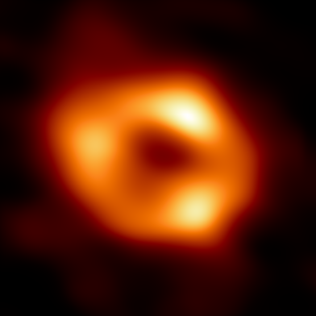
In light of the recent exciting press release about the supermassive black hole at the center of our own Milky Way galaxy, I am going to discuss a brief introduction to black holes and other related concepts in a series of blog articles for those who wish to understand better these amazing monstrous heavenly creatures. For starter, this first article is about Schwarzschild black hole, the simplest black hole model and also the first exact solution of the Einstein’s Field Equation.

The Supermassive Black Hole (Sagittarius A*) at the Center of Milky Way Galaxy.

First, what is a black hole?

A black hole is a hypothetical (though its existence is no longer in doubt) region of spacetime where gravity is so immense that nothing, even light (the lightest matter in the universe) can escape from it.

How did we come to know about a black hole? Was it just an imagination of some mad scientists?

No imagination. We came to know about the theoretical notion of a black hole from Einstein’s general relativity. But long before general relativity came out, French mathematician Pierre-Simon Laplace had already thought about a celestial object whose gravity is so strong that even light can’t escape. It is discussed in his five-volume book Mécanique Céleste (Celestial Mechanics).

In general relativity, black holes are solutions of the Einstein’s Field Equations.

What are the Einstein’s Field Equations?

They are the fundamental equations of Einstein’s theory of gravitation. Such equations are expected to satisfy the following requirements:

  • The field equations should be independent of coordinate systems, i.e. they should be tensorial.
  • They should be partial differential equations of second order for the components $g_{ij}$ of the unknown metric tensor. If you want to know what a metric tensor is, go deeper here.
  • They are a relativistic generalization of the Poisson equation of Newtonian gravitational potential $$\nabla^2\Phi=4\pi G\rho$$ where $\rho$ is the mass density.
  • Since the energy-momentum tensor $T_{ij}$ is the special relativistic analogue of the mass density, it should be the source of the gravitational field.
  • If the space is flat, $T_{ij}$ should vanish.

The equations satisfying all these requirements are given by \begin{equation}\label{eq:EFT}G_{ij}=8\pi GT_{ij}\end{equation} where $G_{ij}=R_{ij}-\frac{1}{2}Rg_{ij}$. $G_{ij}$ is called the Einstein tensor. $R_{ij}$ and $R$ are, respectively, Ricci curvature tensor and scalar curvature. If you want to know what they are, go deeper here. Interestingly, the field equations \eqref{eq:EFT} were derived independently and almost simultaneously by Albert Einstein and David Hilbert in 1915.

So, how do we solve the Field Equations?

The field equations are nonlinear partial differential equations. Partial differential equations are, in general,  difficult to solve with equations alone. We impose additional (physical) assumptions and conditions (such as boundary conditions and initial conditions) so the equations can becomes simpler enough for us to be able to solve. First, we have no information on the source of gravity, i.e. no information on the energy-momentum tensor $T_{ij}$. Instead, we consider the field equations outside the field-producing masses. Thus, we obtain the vacuum field equations $$R_{ij}-\frac{1}{2}Rg_{ij}=0$$ Without loss of generality, we may assume that the metric tensor $g_{ij}$ is diagonal, i.e. $g_{ij}=0$ if $i\ne j$. This results in $R_{ij}=0$ if $i\ne j$ from the vacuum field equations. For $i=j$, since the scalar curvature $R$ is given by $R=\sum_ig^{ii}R_{ii}$, from the vacuum field equations, we have $(n-2)R=0$. For $n=4$, $R=0$ and therefore the vacuum field equations turn into \begin{equation}\label{eq:ricciflat}R_{ij}=0\end{equation} i.e. vanishing Ricci curvature tensor. \eqref{eq:ricciflat} is simpler than the original vacuum field equations but by no means it is easy to solve. The simplest solution of \eqref{eq:ricciflat} was obtained in 1915 by a German physicist Karl Schwarzschild while serving in the army during World War I. This is also the first exact solution to the Einstein’s field equations. Schwarzschild assumed a static spherical symmetric metric as a solution of the vacuum equations \eqref{eq:ricciflat}. The ansatz for a static isotropic metric is given by \begin{equation}\label{eq:ansatz}ds^2=-A(r)dt^2+B(r)dr^2+r^2(d\theta^2+\sin^2\theta d\phi^2)\end{equation} In addition, we want the solution to become the flat spacetime far away from the masses i.e. the solution is asymptotically flat, so we require $$\lim_{r\to\infty}A(r)=\lim_{r\to\infty}B(r)=1$$ Now, we are ready to solve the vacuum field equations \eqref{eq:ricciflat}. From the ansatz \eqref{eq:ansatz}, we have $$g_{tt}=-A(r),\ g_{rr}=B(r),\ g_{\theta\theta}=r^2,\ g_{\phi\phi}=r^2\sin^2\theta$$ The nonzero Christoffel symbols are computed to be \begin{align*}\Gamma_{rr}^r&=\frac{B’}{2B},\ \Gamma_{tt}^r=\frac{A’}{2B},\ \Gamma_{\theta\theta}^r=-\frac{r}{B}\\\Gamma_{\phi\phi}^r&=-\frac{r\sin^2\theta}{B},\ \Gamma_{\theta r}^\theta=\Gamma_{\phi r}^\phi=\frac{1}{r},\\\Gamma_{tr}^t&=\frac{A’}{2A},\ \Gamma_{\phi\phi}^\theta=-\sin\theta\cos\theta,\ \Gamma_{\phi\theta}^\phi=\cot\theta\end{align*} Here, ‘ stands for $\frac{d}{dr}$. Using these Christoffel symbols, the Ricci tensors are computed to be \begin{align*}R_{tt}&=\frac{A^{\prime\prime}}{2B}-\frac{A’}{4B}\left(\frac{A’}{A}+\frac{B’}{B}\right)+\frac{A’}{rB}\\R_{rr}&=-\frac{A^{\prime\prime}}{2A}+\frac{A’}{4A}\left(\frac{A’}{A}+\frac{B’}{B}\right)+\frac{B’}{rB}\\R_{\theta\theta}&=1-\frac{1}{B}-\frac{r}{2B}\left(\frac{A’}{A}-\frac{B’}{B}\right)\\R_{\phi\phi}&=\sin^2\theta R_{\theta\theta}\end{align*} From the first two equations of the Ricci tensors above and by requirung them to be 0, $$BR_{tt}+AR_{rr}=\frac{1}{rB}(A’B+AB’)=\frac{1}{rB}(AB)’=0$$ So, we have $A(r)B(r)$=constant. Asymptotic flatness implies that $A(r)B(r)=1$. $R_{\theta\theta}=0$ along with $B(r)=\frac{1}{A(r)}$ and $A’B+AB’=0$ results in $A+rA’=(rA)’=1$. Hence, $A(r)=1+\frac{C}{r}$, where $C$ is a constant. By weak field approximation (Newtonian limit) , we obtain \begin{align*}A(r)=-g_{00}&=1+\frac{2\Phi}{c^2}\\&=1-\frac{2MG}{c^2r}\end{align*} where $\Phi=-\frac{GM}{r}$. This determines the constant $C=-\frac{2MG}{c^2r}$. Finally, the Schwarzschild solution is given by \begin{equation}\label{eq:bh}ds^2=-\left(1-\frac{2MG}{c^2r}\right)c^2dt^2+\left(1-\frac{2MG}{c^2r}\right)^{-1}dr^2+r^2(d\theta^2+\sin^2\theta d\phi^2)\end{equation} As I mentioned in the beginning, this is the simplest black hole model and also is the first exact solution of the Einstein’s Field Equations. It turns out that Schwarzschild solution is the only spherically symmetric solution to the vacuum Einstein equation \eqref{eq:ricciflat} due to

Birkhoff’s Theorem

In 1923, George David Birkhoff proved:

Theorem. Any spherically symmetric solution of the vacuum Einstein’s field equations \eqref{eq:ricciflat} must be static and asymptotically flat.

The Shape of a Black Hole

Is the converse of Birkhoff’s theorem true? Namely, is any static and asymptotically flat solution of the vacuum field equations necessarily spherically symmetric? I don’t know the answer, though I assume the answer is known. While the notion of a black hole originated from general relativity as a solution of the field equations, general relativity does not tell us how a black hole can be actually formed. A mechanism of black hole formation was provided by nuclear physics as a consequence of the gravitational collapse of a dead star. From our observations of the shape of massive objects , one would think the shape of a black hole is a sphere also. Since we don’t know (I mean I don’t know) for sure, it would be interesting to ponder whether the shape of a black hole different from a sphere can exist, for example a toroidal (doughnut shaped) black hole. If not for Schwarzschild black hole, how about for a rotational black hole?

The Event Horizon

I conclude this article by mentioning that the Schwarzschild solution in \eqref{eq:bh} only describes the outside of the black hole. What determines the inside and the outside of a black hole? It is the event horizon. The event horizon is where $r=r_g=\frac{2MG}{c^2}$. $r_g$ is called the Schwarzschild radius.The Schwarzschild solution requires that $r>r_g$. The Schwarzschild solution unfortunately does not tell anything about whatever happens inside the black hole. We will never know for sure what happens once an object falls into a black hole past its event horizon unless we have information on the source of its gravity, i.e. the stress-energy tensor $T_{ij}$.

The Curvature

In this note, we study different notions of curvatures of a Riemannian or a pseudo-Riemannian $n$-manifold $M$ with metric tensor $g_{ij}$. This note is intended mainly for students of physics. Hence, we will discuss only local expressions of curvatures as those are the ones we mostly use for doing physics in general relativity.

First we need to introduce the Christoffel symbols $\Gamma_{ij}^k$. The Christoffel symbols are associated with the differentiation of vector fields in a Riemannian or a pseudo Riemannian manifold $M$, called the Levi-Civita connection. The Levi-Civita connection $\nabla$ is a generalization of the covariant derivative of vector fields in the Euclidean space. Locally the Levi-civita connection is defined by $$\nabla_{\frac{\partial}{\partial x^i}}\frac{\partial}{\partial x^j}=\sum_{k}\Gamma_{ij}^k\frac{\partial}{\partial x^k}$$ and the Christoffel symbol is given by $$\Gamma_{ij}^k=\frac{1}{2}\sum_\ell g^{k\ell}\left\{\frac{\partial g_{j\ell}}{\partial x^i}+\frac{\partial g_{\ell i}}{\partial x^j}-\frac{\partial g_{ij}}{\partial x^\ell}\right\}$$ where $g^{k\ell}$ is the inverse of the metric tensor.

Locally the Riemann curvature tensor $R_{ijk}^\ell$ is given by $$R_{ijk}^\ell=\frac{\partial}{\partial x^j}\Gamma_{ik}^\ell-\frac{\partial}{\partial x^k}\Gamma_{ij}^\ell+\sum_p\left\{\Gamma_{jp}^\ell\Gamma_{ik}^p-\Gamma_{kp}^\ell\Gamma_{ij}^p\right\}$$

Locally the sectional curvature $K(X,Y)$ of $M$ with respect to the plane spanned by tangent vectors $X,Y\in T_pM$ is given by \begin{equation}\label{eq:sectcurv}K_p(X,Y)=g^{ii}R_{iji}^j\end{equation} assuming that $X,Y\in\mathrm{span}\left\{\frac{\partial}{\partial x^i},\frac{\partial}{\partial x^j}\right\}$. The sectional curvature is a generalization of the Gaußian curvature of a surface in 3-space. To see this, let $\varphi: M^2\longrightarrow M^3$ be a conformal parametric surface $M^2$ immersed in 3-space $M^3$ with metric $e^{u(x,y)}(dx^2+dy^2)$. The Gaußian curvature $K$ of $\varphi$ can be calculated using the formula (due to Karl Friedrich Gauß) $$K=\frac{\ell n-m^2}{EG-F^2}$$ where \begin{align*}E&=\langle\varphi_x,\varphi_x\rangle,\ F=\langle\varphi_x,\varphi_y\rangle,\ G=\langle\varphi_y,\varphi_y\rangle,\\\ell&=\langle\varphi_{xx},N\rangle,\ m=\langle\varphi_{xy},N\rangle,\ n=\langle\varphi_{yy},N\rangle\end{align*} Here, $\langle\ ,\ \rangle$ stands for the inner product induced by the conformal metric $e^{u(x,y)}(dx^2+dy^2)$ and $N$ is the unit normal vector field on $\varphi$. The Gaußian curvature is then obtained as the Liouville’s partial differential equation \begin{equation}\label{eq:liouville}\nabla^2 u=-2Ke^u\end{equation} On the other hand, using \eqref{eq:sectcurv} we find the sectional curvature of $\varphi$ to be $$g^{11}R_{121}^2=-\frac{e^{u(x,y)}}{2}\nabla^2u$$ which coincides with the Gaußian curvature $K$ from \eqref{eq:liouville}

Example. Let us compute the sectional curvature of the hyperbolic plane $$\mathbb{H}^2=\{(x,y)\in\mathbb{R}^2: y>0\}$$ with metric $$ds^2=\frac{dx^2+dy^2}{y^2}$$

The metric tensor is $(g_{ij})=\begin{pmatrix}\frac{1}{y^2} & 0\\0 & \frac{1}{y^2}\end{pmatrix}$. The Riemann curvature tensor $R_{121}^2$ is \begin{align*}R_{121}^2&=\frac{\partial}{\partial y}\Gamma_{11}^2-\frac{\partial}{\partial x}\Gamma_{12}^2+\sum_p\{\Gamma_{2p}^p\Gamma_{11}^p-\Gamma_{1p}^2\Gamma_{12}^p\}\\&=\frac{\partial}{\partial y}\Gamma_{11}^2-\frac{\partial}{\partial x}\Gamma_{12}^2+\Gamma_{21}^2\Gamma_{11}^1-\Gamma_{11}^2\Gamma_{12}^1+\Gamma_{22}^2\Gamma_{11}^2-\Gamma_{12}^2\Gamma_{12}^2\end{align*} We find the Christoffel symbols $$\Gamma_{11}^2=\frac{1}{y},\ \Gamma_{12}^1=-\frac{1}{y},\ \Gamma_{12}^2=0,\ \Gamma_{21}^2=0,\ \Gamma_{22}^2=-\frac{1}{y}$$ Thus we obtain $R_{121}^2=-\frac{1}{y^2}$ and hence $\mathbb{H}^2$ has the constant negative sectional curvature $$K=g^{11}R_{121}^2=y^2\left(-\frac{1}{y^2}\right)=-1$$ What is the shortest path connecting two points $(x_1,y_1)$ and $(x_2,y_2)$ in $\mathbb{H}^2$? Such shortest paths are called geodesics in differential geometry. To find out what a geodesic in $\mathbb{H}^2$ looks like, let $$J=\int_{(x_1,y_1)}^{(x_2,y_2)}ds=\int_{(x_1,y_1)}^{(x_2,y_2)}\frac{\sqrt{1+y_x^2}}{y}dx$$ where $y_x=\frac{dy}{dx}$. The shortest path would satisfy the Euler-Lagrange equation \begin{equation}\label{eq:E-L}\frac{\partial f}{\partial x}-\frac{d}{dx}\left(f-y_x\frac{\partial f}{\partial y_x}\right)=0\end{equation}with $f(y,y_x,x)=\frac{\sqrt{1+y_x^2}}{y}$. Since $f$ does not depend on $x$, $\frac{\partial f}{\partial x}=0$ and the Euler-Lagrange equation \eqref{eq:E-L} becomes $$\frac{d}{dx}\left[\frac{1}{y\sqrt{1+y_x^2}}\right]=0$$ i.e. \begin{equation}\label{eq:E-L2}\frac{1}{y\sqrt{1+y_x^2}}=C\end{equation} where $C$ is a constant. The equation \eqref{eq:E-L2} results in a separable differential equation $$\frac{dy}{dx}=\frac{\sqrt{r^2-y^2}}{y}$$ where $r^2=\frac{1}{C}$. The solution of this equation is $$(x-a)^2+y^2=r^2$$ where $a$ is a constant. Since $y>0$, the solution represents an equation of upper semi circle centered at $(a,0)$ with radius $r$, that is the shortest path (geodesic) between two points $(x_1,y_1)$ and $(x_2,y_2)$ in $\mathbb{H}^2$ is a part of an upper semicircle joining them. In particular, if $x_1=x_2$, the geodesic between $(x_1,y_1)$ and $(x_2,y_2)$ is the vertical line passing through the two points. Such a vertical line can still be considered as an upper semicircle with radius $\infty$.

Geodesics in Hyperbolic Plane

Two other notions of curvatures are Ricci and scalar curvatures. The Ricci curvature tensor is given by $$\mathrm{Ric}_p\left(\frac{\partial}{\partial x^i},\frac{\partial}{\partial x^j}\right)=\sum_kR_{ikj}^k$$ We usually denote $\mathrm{Ric}_p\left(\frac{\partial}{\partial x^i},\frac{\partial}{\partial x^j}\right)$ simply by $R_{ij}$. The scalar curvature $\mathrm{Scal}(p)$ is given by $$\mathrm{Scal}(p)=\sum_{i}g^{ii}R_{ii}$$ The scalar curvature can be given, in terms of the sectional curvature, by $$\mathrm{Scal}(p)=\sum_{i\ne j}K_p\left(\frac{\partial}{\partial x^i},\frac{\partial}{\partial x^j}\right)$$ The scalar curvature is usually denoted by $R$ in general relativity.

Definition. A Riemannian or a pseudo-Riemannian manifold $(M,g)$ is said to be maximally symmetric if $(M,g)$ has constant sectional curvature $\kappa$.

Theorem. If a Riemannian or a pseudo-Riemannian manifold $(M,g)$ is maximally symmetric, then $$R_{ii}=\kappa(n-1)g_{ii}$$ where $\kappa$ is the constant sectional curvature of $(M,g)$ and $n=\dim M$.

Corollary. If $(M,g)$ has the constant sectional curvature $\kappa$, then $$\mathrm{Scal}(p)=n(n-1)\kappa$$ where $n=\dim M$.

Riemannian and Pseudo-Riemannian Manifolds

This note is intended particularly for students of physics who have never had any prior encounter with differential geometry. Hence, I try to maintain mathematical rigor and technicalities at a minimum when I discuss differential geometric concepts, instead mostly use hand-waving and rudimentary arguments with emphases on physical ideas and intuition.

The notion of (pseudo-)Riemannian manifolds plays an important role in studying general relativity. But first, what is a manifold? A manifold is, very roughly speaking, a space which locally looks like our space (Euclidean space). In other words, for any point $p$ in a manifold $M$ there exists a neighborhood (called a coordinate neighborhood) $U$ of $p$ such that $U\cong\mathbb{R}^n$. Here $\cong$ means they are homeomorphic i.e. topologically indistinguishable. Such a property is said to be locally Euclidean and a space which is locally $\mathbb{R}^n$ is called an $n$-dimensional manifold. Actually being locally Euclidean is not the only condition for a space to be a manifold but that is the most important property of a manifold for physicists.

Figure 1, A manifold

Figure 1 shows a manifold $M$, two coordinate neighborhood $U$ and $V$ with homeomorphisms $\phi$ and $\psi$, respectively. Why do we need manifolds by the way? In order to do physics, we need coordinates. Without coordinates we can’t write equations of motion. Unfortunately, even for a simple familiar space there is no guarantee that there will be a global coordinate system. Here is an example.

Example. The points $(x,y,z)$ on the 2-sphere $S^2$ are represented in terms of the spherical coordinates $(\theta,\phi)$ as $$x=\sin\phi\cos\theta,\ y=\sin\phi\sin\theta,\ z=\cos\phi,\ 0\leq\phi\leq\pi,\ 0\leq\theta\leq 2\pi$$ Using the chain rule, we can write the standard basis $\frac{\partial}{\partial\theta}$, $\frac{\partial}{\partial\phi}$ for the tangent space $T_\ast S^2$ in spherical coordinates in terms of the standard basis $\frac{\partial}{\partial x}$, $\frac{\partial}{\partial y}$, $\frac{\partial}{\partial y}$ in rectangular coordinates as \begin{align*}\frac{\partial}{\partial\theta}&=-\sin\phi\sin\theta\frac{\partial}{\partial x}+\sin\phi\cos\theta\frac{\partial}{\partial y}\\\frac{\partial}{\partial\phi}&=\cos\phi\cos\theta\frac{\partial}{\partial x}+\cos\phi\sin\theta\frac{\partial}{\partial y}-\sin\phi\frac{\partial}{\partial z}\end{align*} This frame field is not globally defined on $S^2$ because $\frac{\partial}{\partial\theta}=0$ at $\phi=0,\pi$ i.e. at the north pole $N=(0,0,1)$ and at the south pole $S=(0,0,-1)$ as also seen in Figure 2.

Figure 2. The 2-sphere with frame field

The 2-sphere $S^2$ is covered by two coordinates neighborhoods $U=S^2\setminus{N}$ and $V=S^2\setminus{S}$, each of which is identified with $\mathbb{R}^2$, the Euclidean plane via the stereographic projection. Figure 3 shows the stereographic projection from the north pole $N$, which is a one-to-one correspondence from $U$ to $\mathbb{R}^2$.

Figure 3. The Stereographic Projection

A global coordinate system exists in the flat Euclidean space (or a flat pseudo-Euclidean space including Minkowski spacetime), however general relativity has taught us that a physical space is not necessarily a flat space (vaccum spacetime). This is where a manifold comes in. A manifold guarantees the existence coordinate system at least locally and for most cases that is good enough to do physics in particular we write physical equations in a coordinate independent way, so that if a physical equation holds in on coordinate neighborhood, it should also hold in another coordinate neighborhood in the same way.

We would be needing more than topological manifolds to do physics. For an obvious reason we need differentiable manifolds. I am not going to delve into this except for just saying that a differentiable manifold is a manifold on which the differentiability of functions and vector fields can be defined and also to which tangent space at each point can be considered. (If we can’t differentiate fields, we cannot do physics.) In addition, we need Riemannian manifolds. A Riemannian manifold is a differentiable manifold with a Riemannian metric. So what is a Riemannian metric? A Riemannian metric $g$ is a positive definite bilinear symmetric form $g_p: T_pM\times T_pM\longrightarrow\mathbb{R}$, which induces a positive definite inner product on each tangent space $T_pM$. In a  coordinate neighborhood, the metric $g$ can be locally given by \begin{equation}\label{eq:metric}g=g_{ij}dx^i\otimes dx^j\end{equation}Here we are using the Einstein’s summation convention. The  $n\times n$ matrix $(g_{ij})$ is called a metric tensor and physicists often simply write $g_{ij}$ for the metric tensor, not for the component. Since $g_{ij}$ is a symmetric tensor, it can be diagonalized. Since the metric is preserved under diagonalization (which amounts to a change of coordinates), without loss of generality we may assume that $g_{ij}=0$ if $i\ne j$ so that the metric tensor \eqref{eq:metric} is written as\begin{equation}\label{eq:metric2}g=g_{ii}dx^i\otimes dx^i\end{equation}Let the dimension of $M$ be $n$. Then each tangent space $T_pM$ is an $n$-dimensional vector space with the canonical orthonormal basis $\left(\frac{\partial}{\partial x^1}\right)_p,\cdots,\left(\frac{\partial}{\partial x^n}\right)_p$. Thus any tangent vector $v\in T_pM$ can be written as $$v=v^j\left(\frac{\partial}{\partial x^j}\right)_p$$ The differential 1-forms $d^i$ are the duals of $\frac{\partial}{\partial x^i}$, respectively. $$dx^i\left(\frac{\partial}{\partial x^j}\right)=\delta_{ij}$$ and hence $$dx^i(v)=v^i$$ For any two tangent vectors $v,w\in T_pM$ using \eqref{eq:metric2} we obtain \begin{equation}\label{eq:metric3}g(v,w)=g_{ii}dx^i\otimes dx^i(v,w)=g_{ii}dx^i(v)dx^i(w)=g_{ii}v^iw^i\end{equation}\eqref{eq:metric3} shows how the metric $g$ induces an inner product on each tangent space $T_pM$. In doing physics, in particular general relativity, the physical space is often a pseudo-Riemannian manifold rather than a Riemannian manifold. A pseudo-Riemannian manifold is equipped with a pseudo-Riemannian metric which is an indefinite symmetric bilinear form. So the induced inner product is indefinite. A good example is the Minkowski spacetime $\mathbb{R}^{3+1}$ which is $\mathbb{R}^4$ with the Minkowski metric or the Lorentz-Minkowski metric \begin{equation}\label{eq:minkowski}g=-dt^2+dx^2+dy^2+dz^2\end{equation} The Minkowski metric \eqref{eq:minkowski} induces the inner product on $\mathbb{R}^{3+1}$ (The Minkowski spacetime has a single coordinate neighborhood $\mathbb{R}^{3+1}$ itself and every tangent space $T_p\mathbb{R}^{3+1}$ is isomorphic to $\mathbb{R}^{3+1}$, hence $\mathbb{R}^{3+1}$ is a manifold and at the same time it is also a vector space.) $$\langle v,w\rangle=-v^0w^0+v^1w^1+v^2w^2+v^3w^3$$ where $v=(v^0,v^1,v^2,v^3)$ and $w=(w^0,w^1,w^2,w^3)$ are four-vectors in $\mathbb{R}^{3+1}$.

In conclusion, I would like to emphasize that the metric tensor $g_{ij}$ is the most important ingredient of a Riemannian or a pseudo-Riemannian manifold. You can literally find out everything about the geometry of a Riemannian or a pseudo-Riemannian manifold with the metric tensor. With the metric tensor, you can also find out about what gravity does when there is matter (the source of gravity) present in the manifold.