Category Archives: Differential Geometry

The Diagonalization of a Riemannian Metric

Let $(M^n, ds^2)$ denote an $n$-dimensional Riemannian manifold. The Riemannian metric $ds^2$, in general, is given, in terms of local coordinates $x’_1,\cdots,x’_n$, by $$ds^2=\sum_{i,j}h_{ij}(x’_1,\cdots,x’_n)dx’_idx’_j$$ Since the metric tensor $(h_{ij})$ is symmetric, by the finite dimensional spectral theorem, there exists an orthogonal matrix $O$ such that $O^t(h_{ij})O=(g_{ii})$. Let $$\begin{pmatrix}dx_1\\\vdots\\dx_n\end{pmatrix}=O^t\begin{pmatrix}dx’_1\\\vdots\\dx’_n\end{pmatrix}$$ Then \begin{align*}ds^2&=\sum_{i,j}h_{ij}(x’_1,\cdots,x’_n)dx’_idx’_j\\&=\begin{pmatrix}dx’_1\\\vdots\\dx’_n\end{pmatrix}^t(h_{ij})\begin{pmatrix}dx’_1\\\vdots\\dx’_n\end{pmatrix}\\&=\left[O\begin{pmatrix}dx_1\\\vdots\\dx_n\end{pmatrix}\right]^tO(g_{ii})O^t\left[O\begin{pmatrix}dx_1\\\vdots\\dx_n\end{pmatrix}\right]\\&=\begin{pmatrix}dx_1\\\vdots\\dx_n\end{pmatrix}^t(g_{ii})\begin{pmatrix}dx_1\\\vdots\\dx_n\end{pmatrix}\\&=\sum_{i}g_{ii}dx_i^2\end{align*} Therefore, without loss of generality, we may assume that a Riemannian metric is of the diagonal form $$ds^2=\sum_{i}g_{ii}(x_1,\cdots,x_n)dx_i^2$$

The Curvature

In this note, we study different notions of curvatures of a Riemannian or a pseudo-Riemannian $n$-manifold $M$ with metric tensor $g_{ij}$. This note is intended mainly for students of physics. Hence, we will discuss only local expressions of curvatures as those are the ones we mostly use for doing physics in general relativity.

First we need to introduce the Christoffel symbols $\Gamma_{ij}^k$. The Christoffel symbols are associated with the differentiation of vector fields in a Riemannian or a pseudo Riemannian manifold $M$, called the Levi-Civita connection. The Levi-Civita connection $\nabla$ is a generalization of the covariant derivative of vector fields in the Euclidean space. Locally the Levi-civita connection is defined by $$\nabla_{\frac{\partial}{\partial x^i}}\frac{\partial}{\partial x^j}=\sum_{k}\Gamma_{ij}^k\frac{\partial}{\partial x^k}$$ and the Christoffel symbol is given by $$\Gamma_{ij}^k=\frac{1}{2}\sum_\ell g^{k\ell}\left\{\frac{\partial g_{j\ell}}{\partial x^i}+\frac{\partial g_{\ell i}}{\partial x^j}-\frac{\partial g_{ij}}{\partial x^\ell}\right\}$$ where $g^{k\ell}$ is the inverse of the metric tensor.

Locally the Riemann curvature tensor $R_{ijk}^\ell$ is given by $$R_{ijk}^\ell=\frac{\partial}{\partial x^j}\Gamma_{ik}^\ell-\frac{\partial}{\partial x^k}\Gamma_{ij}^\ell+\sum_p\left\{\Gamma_{jp}^\ell\Gamma_{ik}^p-\Gamma_{kp}^\ell\Gamma_{ij}^p\right\}$$

Locally the sectional curvature $K(X,Y)$ of $M$ with respect to the plane spanned by tangent vectors $X,Y\in T_pM$ is given by \begin{equation}\label{eq:sectcurv}K_p(X,Y)=g^{ii}R_{iji}^j\end{equation} assuming that $X,Y\in\mathrm{span}\left\{\frac{\partial}{\partial x^i},\frac{\partial}{\partial x^j}\right\}$. The sectional curvature is a generalization of the Gaußian curvature of a surface in 3-space. To see this, let $\varphi: M^2\longrightarrow M^3$ be a conformal parametric surface $M^2$ immersed in 3-space $M^3$ with metric $e^{u(x,y)}(dx^2+dy^2)$. The Gaußian curvature $K$ of $\varphi$ can be calculated using the formula (due to Karl Friedrich Gauß) $$K=\frac{\ell n-m^2}{EG-F^2}$$ where \begin{align*}E&=\langle\varphi_x,\varphi_x\rangle,\ F=\langle\varphi_x,\varphi_y\rangle,\ G=\langle\varphi_y,\varphi_y\rangle,\\\ell&=\langle\varphi_{xx},N\rangle,\ m=\langle\varphi_{xy},N\rangle,\ n=\langle\varphi_{yy},N\rangle\end{align*} Here, $\langle\ ,\ \rangle$ stands for the inner product induced by the conformal metric $e^{u(x,y)}(dx^2+dy^2)$ and $N$ is the unit normal vector field on $\varphi$. The Gaußian curvature is then obtained as the Liouville’s partial differential equation \begin{equation}\label{eq:liouville}\nabla^2 u=-2Ke^u\end{equation} On the other hand, using \eqref{eq:sectcurv} we find the sectional curvature of $\varphi$ to be $$g^{11}R_{121}^2=-\frac{e^{u(x,y)}}{2}\nabla^2u$$ which coincides with the Gaußian curvature $K$ from \eqref{eq:liouville}

Example. Let us compute the sectional curvature of the hyperbolic plane $$\mathbb{H}^2=\{(x,y)\in\mathbb{R}^2: y>0\}$$ with metric $$ds^2=\frac{dx^2+dy^2}{y^2}$$

The metric tensor is $(g_{ij})=\begin{pmatrix}\frac{1}{y^2} & 0\\0 & \frac{1}{y^2}\end{pmatrix}$. The Riemann curvature tensor $R_{121}^2$ is \begin{align*}R_{121}^2&=\frac{\partial}{\partial y}\Gamma_{11}^2-\frac{\partial}{\partial x}\Gamma_{12}^2+\sum_p\{\Gamma_{2p}^p\Gamma_{11}^p-\Gamma_{1p}^2\Gamma_{12}^p\}\\&=\frac{\partial}{\partial y}\Gamma_{11}^2-\frac{\partial}{\partial x}\Gamma_{12}^2+\Gamma_{21}^2\Gamma_{11}^1-\Gamma_{11}^2\Gamma_{12}^1+\Gamma_{22}^2\Gamma_{11}^2-\Gamma_{12}^2\Gamma_{12}^2\end{align*} We find the Christoffel symbols $$\Gamma_{11}^2=\frac{1}{y},\ \Gamma_{12}^1=-\frac{1}{y},\ \Gamma_{12}^2=0,\ \Gamma_{21}^2=0,\ \Gamma_{22}^2=-\frac{1}{y}$$ Thus we obtain $R_{121}^2=-\frac{1}{y^2}$ and hence $\mathbb{H}^2$ has the constant negative sectional curvature $$K=g^{11}R_{121}^2=y^2\left(-\frac{1}{y^2}\right)=-1$$ What is the shortest path connecting two points $(x_1,y_1)$ and $(x_2,y_2)$ in $\mathbb{H}^2$? Such shortest paths are called geodesics in differential geometry. To find out what a geodesic in $\mathbb{H}^2$ looks like, let $$J=\int_{(x_1,y_1)}^{(x_2,y_2)}ds=\int_{(x_1,y_1)}^{(x_2,y_2)}\frac{\sqrt{1+y_x^2}}{y}dx$$ where $y_x=\frac{dy}{dx}$. The shortest path would satisfy the Euler-Lagrange equation \begin{equation}\label{eq:E-L}\frac{\partial f}{\partial x}-\frac{d}{dx}\left(f-y_x\frac{\partial f}{\partial y_x}\right)=0\end{equation}with $f(y,y_x,x)=\frac{\sqrt{1+y_x^2}}{y}$. Since $f$ does not depend on $x$, $\frac{\partial f}{\partial x}=0$ and the Euler-Lagrange equation \eqref{eq:E-L} becomes $$\frac{d}{dx}\left[\frac{1}{y\sqrt{1+y_x^2}}\right]=0$$ i.e. \begin{equation}\label{eq:E-L2}\frac{1}{y\sqrt{1+y_x^2}}=C\end{equation} where $C$ is a constant. The equation \eqref{eq:E-L2} results in a separable differential equation $$\frac{dy}{dx}=\frac{\sqrt{r^2-y^2}}{y}$$ where $r^2=\frac{1}{C}$. The solution of this equation is $$(x-a)^2+y^2=r^2$$ where $a$ is a constant. Since $y>0$, the solution represents an equation of upper semi circle centered at $(a,0)$ with radius $r$, that is the shortest path (geodesic) between two points $(x_1,y_1)$ and $(x_2,y_2)$ in $\mathbb{H}^2$ is a part of an upper semicircle joining them. In particular, if $x_1=x_2$, the geodesic between $(x_1,y_1)$ and $(x_2,y_2)$ is the vertical line passing through the two points. Such a vertical line can still be considered as an upper semicircle with radius $\infty$.

Geodesics in Hyperbolic Plane

Two other notions of curvatures are Ricci and scalar curvatures. The Ricci curvature tensor is given by $$\mathrm{Ric}_p\left(\frac{\partial}{\partial x^i},\frac{\partial}{\partial x^j}\right)=\sum_kR_{ikj}^k$$ We usually denote $\mathrm{Ric}_p\left(\frac{\partial}{\partial x^i},\frac{\partial}{\partial x^j}\right)$ simply by $R_{ij}$. The scalar curvature $\mathrm{Scal}(p)$ is given by $$\mathrm{Scal}(p)=\sum_{i}g^{ii}R_{ii}$$ The scalar curvature can be given, in terms of the sectional curvature, by $$\mathrm{Scal}(p)=\sum_{i\ne j}K_p\left(\frac{\partial}{\partial x^i},\frac{\partial}{\partial x^j}\right)$$ The scalar curvature is usually denoted by $R$ in general relativity.

Definition. A Riemannian or a pseudo-Riemannian manifold $(M,g)$ is said to be maximally symmetric if $(M,g)$ has constant sectional curvature $\kappa$.

Theorem. If a Riemannian or a pseudo-Riemannian manifold $(M,g)$ is maximally symmetric, then $$R_{ii}=\kappa(n-1)g_{ii}$$ where $\kappa$ is the constant sectional curvature of $(M,g)$ and $n=\dim M$.

Corollary. If $(M,g)$ has the constant sectional curvature $\kappa$, then $$\mathrm{Scal}(p)=n(n-1)\kappa$$ where $n=\dim M$.

Riemannian and Pseudo-Riemannian Manifolds

This note is intended particularly for students of physics who have never had any prior encounter with differential geometry. Hence, I try to maintain mathematical rigor and technicalities at a minimum when I discuss differential geometric concepts, instead mostly use hand-waving and rudimentary arguments with emphases on physical ideas and intuition.

The notion of (pseudo-)Riemannian manifolds plays an important role in studying general relativity. But first, what is a manifold? A manifold is, very roughly speaking, a space which locally looks like our space (Euclidean space). In other words, for any point $p$ in a manifold $M$ there exists a neighborhood (called a coordinate neighborhood) $U$ of $p$ such that $U\cong\mathbb{R}^n$. Here $\cong$ means they are homeomorphic i.e. topologically indistinguishable. Such a property is said to be locally Euclidean and a space which is locally $\mathbb{R}^n$ is called an $n$-dimensional manifold. Actually being locally Euclidean is not the only condition for a space to be a manifold but that is the most important property of a manifold for physicists.

Figure 1, A manifold

Figure 1 shows a manifold $M$, two coordinate neighborhood $U$ and $V$ with homeomorphisms $\phi$ and $\psi$, respectively. Why do we need manifolds by the way? In order to do physics, we need coordinates. Without coordinates we can’t write equations of motion. Unfortunately, even for a simple familiar space there is no guarantee that there will be a global coordinate system. Here is an example.

Example. The points $(x,y,z)$ on the 2-sphere $S^2$ are represented in terms of the spherical coordinates $(\theta,\phi)$ as $$x=\sin\phi\cos\theta,\ y=\sin\phi\sin\theta,\ z=\cos\phi,\ 0\leq\phi\leq\pi,\ 0\leq\theta\leq 2\pi$$ Using the chain rule, we can write the standard basis $\frac{\partial}{\partial\theta}$, $\frac{\partial}{\partial\phi}$ for the tangent space $T_\ast S^2$ in spherical coordinates in terms of the standard basis $\frac{\partial}{\partial x}$, $\frac{\partial}{\partial y}$, $\frac{\partial}{\partial y}$ in rectangular coordinates as \begin{align*}\frac{\partial}{\partial\theta}&=-\sin\phi\sin\theta\frac{\partial}{\partial x}+\sin\phi\cos\theta\frac{\partial}{\partial y}\\\frac{\partial}{\partial\phi}&=\cos\phi\cos\theta\frac{\partial}{\partial x}+\cos\phi\sin\theta\frac{\partial}{\partial y}-\sin\phi\frac{\partial}{\partial z}\end{align*} This frame field is not globally defined on $S^2$ because $\frac{\partial}{\partial\theta}=0$ at $\phi=0,\pi$ i.e. at the north pole $N=(0,0,1)$ and at the south pole $S=(0,0,-1)$ as also seen in Figure 2.

Figure 2. The 2-sphere with frame field

The 2-sphere $S^2$ is covered by two coordinates neighborhoods $U=S^2\setminus{N}$ and $V=S^2\setminus{S}$, each of which is identified with $\mathbb{R}^2$, the Euclidean plane via the stereographic projection. Figure 3 shows the stereographic projection from the north pole $N$, which is a one-to-one correspondence from $U$ to $\mathbb{R}^2$.

Figure 3. The Stereographic Projection

A global coordinate system exists in the flat Euclidean space (or a flat pseudo-Euclidean space including Minkowski spacetime), however general relativity has taught us that a physical space is not necessarily a flat space (vaccum spacetime). This is where a manifold comes in. A manifold guarantees the existence coordinate system at least locally and for most cases that is good enough to do physics in particular we write physical equations in a coordinate independent way, so that if a physical equation holds in on coordinate neighborhood, it should also hold in another coordinate neighborhood in the same way.

We would be needing more than topological manifolds to do physics. For an obvious reason we need differentiable manifolds. I am not going to delve into this except for just saying that a differentiable manifold is a manifold on which the differentiability of functions and vector fields can be defined and also to which tangent space at each point can be considered. (If we can’t differentiate fields, we cannot do physics.) In addition, we need Riemannian manifolds. A Riemannian manifold is a differentiable manifold with a Riemannian metric. So what is a Riemannian metric? A Riemannian metric $g$ is a positive definite bilinear symmetric form $g_p: T_pM\times T_pM\longrightarrow\mathbb{R}$, which induces a positive definite inner product on each tangent space $T_pM$. In a  coordinate neighborhood, the metric $g$ can be locally given by \begin{equation}\label{eq:metric}g=g_{ij}dx^i\otimes dx^j\end{equation}Here we are using the Einstein’s summation convention. The  $n\times n$ matrix $(g_{ij})$ is called a metric tensor and physicists often simply write $g_{ij}$ for the metric tensor, not for the component. Since $g_{ij}$ is a symmetric tensor, it can be diagonalized. Since the metric is preserved under diagonalization (which amounts to a change of coordinates), without loss of generality we may assume that $g_{ij}=0$ if $i\ne j$ so that the metric tensor \eqref{eq:metric} is written as\begin{equation}\label{eq:metric2}g=g_{ii}dx^i\otimes dx^i\end{equation}Let the dimension of $M$ be $n$. Then each tangent space $T_pM$ is an $n$-dimensional vector space with the canonical orthonormal basis $\left(\frac{\partial}{\partial x^1}\right)_p,\cdots,\left(\frac{\partial}{\partial x^n}\right)_p$. Thus any tangent vector $v\in T_pM$ can be written as $$v=v^j\left(\frac{\partial}{\partial x^j}\right)_p$$ The differential 1-forms $d^i$ are the duals of $\frac{\partial}{\partial x^i}$, respectively. $$dx^i\left(\frac{\partial}{\partial x^j}\right)=\delta_{ij}$$ and hence $$dx^i(v)=v^i$$ For any two tangent vectors $v,w\in T_pM$ using \eqref{eq:metric2} we obtain \begin{equation}\label{eq:metric3}g(v,w)=g_{ii}dx^i\otimes dx^i(v,w)=g_{ii}dx^i(v)dx^i(w)=g_{ii}v^iw^i\end{equation}\eqref{eq:metric3} shows how the metric $g$ induces an inner product on each tangent space $T_pM$. In doing physics, in particular general relativity, the physical space is often a pseudo-Riemannian manifold rather than a Riemannian manifold. A pseudo-Riemannian manifold is equipped with a pseudo-Riemannian metric which is an indefinite symmetric bilinear form. So the induced inner product is indefinite. A good example is the Minkowski spacetime $\mathbb{R}^{3+1}$ which is $\mathbb{R}^4$ with the Minkowski metric or the Lorentz-Minkowski metric \begin{equation}\label{eq:minkowski}g=-dt^2+dx^2+dy^2+dz^2\end{equation} The Minkowski metric \eqref{eq:minkowski} induces the inner product on $\mathbb{R}^{3+1}$ (The Minkowski spacetime has a single coordinate neighborhood $\mathbb{R}^{3+1}$ itself and every tangent space $T_p\mathbb{R}^{3+1}$ is isomorphic to $\mathbb{R}^{3+1}$, hence $\mathbb{R}^{3+1}$ is a manifold and at the same time it is also a vector space.) $$\langle v,w\rangle=-v^0w^0+v^1w^1+v^2w^2+v^3w^3$$ where $v=(v^0,v^1,v^2,v^3)$ and $w=(w^0,w^1,w^2,w^3)$ are four-vectors in $\mathbb{R}^{3+1}$.

In conclusion, I would like to emphasize that the metric tensor $g_{ij}$ is the most important ingredient of a Riemannian or a pseudo-Riemannian manifold. You can literally find out everything about the geometry of a Riemannian or a pseudo-Riemannian manifold with the metric tensor. With the metric tensor, you can also find out about what gravity does when there is matter (the source of gravity) present in the manifold.

The interior area of a simple closed curve is invariant under a rigid motion

Let $\gamma(t)=(x(t),y(t))$ be a positively-oriented simple closed curve in $\mathbb{R}^2$ with period $a$. The area of its interior is given by
$$A(\mathrm{int}(\gamma))=\int\int_{\mathrm{int}(\gamma)}dxdy=\frac{1}{2}\int_0^a(x\dot y-y\dot x)dt$$
The last line integral is obtained by applying Green’s Theorem to the second double integral. A rigid motion can be given by $M=T_b\circ R_{\theta}$ where $R_{\theta}=\begin{pmatrix}
\cos\theta & -\sin\theta\\
\sin\theta & \cos\theta
\end{pmatrix}$ is a rotation by an angle $\theta$ and $T_b$ is a translation by a constant vector $b=(b_1,b_2)$. So $\tilde\gamma=M(\gamma)$ is given by
$$\tilde\gamma=(\tilde x,\tilde y)=(x\cos\theta-y\sin\theta+b_1,x\sin\theta+y\cos\theta+b_2)$$
and
\begin{align*}\tilde x\dot{\tilde y}-\tilde y\dot{\tilde x}&=x\dot y-y\dot x+b_1(\dot x\sin\theta+\dot y\cos\theta)-b_2(\dot x\cos\theta-\dot y\sin\theta)\\&=x\dot y-y\dot x+b\cdot\begin{pmatrix}
\sin\theta & \cos\theta\\
-\cos\theta & \sin\theta
\end{pmatrix}\begin{pmatrix}
\dot x\\
\dot y
\end{pmatrix}\\&=x\dot y-y\dot x+b\cdot R_{\theta-\frac{\pi}{2}}(\dot\gamma)\end{align*}
\begin{align*}\int_0^a b\cdot R_{\theta-\frac{\pi}{2}}(\dot\gamma(t))dt&=b\cdot R_{\theta-\frac{\pi}{2}}\left(\int_0^a\dot\gamma(t)dt\right)\\
&=0\end{align*}
since $\int_0^a\dot\gamma(t)dt=\gamma(a)-\gamma(0)=0$. ($\gamma(t)$ is a simple closed curve with period $a$.) Therefore, $A(\mathrm{int}(\gamma))=A(\mathrm{int}(M(\gamma))$.

The Curvature of a Surface in Euclidean 3-Space $\mathbb{R}^3$

In here, it is seen that the curvature of a unit speed parametric curve $\alpha(t)$ in $\mathbb{R}^3$ can be measured by its acceleration $\ddot\alpha(t)$. In this case, the acceleration happens to be a normal vector field along the curve. Now we turn our attention to surfaces in Euclidean 3-space $\mathbb{R}^3$ and we would like to devise a way to measure the bending of a surface in $\mathbb{R}^3$, and it may be achieved by studying the change of a unit normal vector field on the surface. To study the change of a unit normal vector field on a surface, we need to be able to differentiate vector fields. But first let us review the directional derivative you learned in mutilvariable calculus. Let $f:\mathbb{R}^3\longrightarrow\mathbb{R}$ be a differentiable function and $\mathbf{v}$ a tangent vector to $\mathbb{R}^3$ at $\mathbf{p}$. Then the directional derivative of $f$ in the $\mathbf{v}$ direction at $\mathbf{p}$ is defined by
\begin{equation}
\label{eq:directderiv}
\nabla_{\mathbf{v}}f=\left.\frac{d}{dt}f(\mathbf{p}+t\mathbf{v})\right|_{t=0}.
\end{equation}
By chain rule, the directional derivative can be written as
\begin{equation}
\label{eq:directderiv2}
\nabla_{\mathbf{v}}f=\nabla f(\mathbf{p})\cdot\mathbf{v},
\end{equation}
where $\nabla f$ denotes the gradient of $f$
$$\nabla f=\frac{\partial f}{\partial x_1}E_1(\mathbf{p})+\frac{\partial f}{\partial x_2}E_2(\mathbf{p})+\frac{\partial f}{\partial x_3}E_3(\mathbf{p}),$$
where $E_1, E_2, E_3$ denote the standard orthonormal frame in $\mathbb{R}^3$. The directional derivative satisfies the following properties.

Theorem. Let $f,g$ be real-valued differentiable functions on $\mathbb{R}^3$, $\mathbf{v},\mathbf{w}$ tangent vectors to $\mathbb{R}^3$ at $\mathbf{p}$, and $a,b\in\mathbb{R}$. Then

  1. $\nabla_{a\mathbf{v}+b\mathbf{w}}f=a\nabla_{\mathbf{v}}f+b\nabla_{\mathbf{w}}f$
  2. $\nabla_{\mathbf{v}}(af+bg)=a\nabla_{\mathbf{v}}f+b\nabla_{\mathbf{v}}g$
  3. $\nabla_{\mathbf{v}}fg=(\nabla_{\mathbf{v}}f)g(\mathbf{p})+f(\mathbf{p})\nabla_{\mathbf{v}}g$

The properties 1 and 2 are linearity and the property 3 is Leibniz rule. The directional derivative \eqref{eq:directderiv} can be generalized to the covariant derivative $\nabla_{\mathbf{v}}X$ of a vector field $X$ in the direction of a tangent vector $\mathbf{v}$ at $\mathbf{p}$:
\begin{equation}
\label{eq:covderiv}
\nabla_{\mathbf{v}}X=\left.\frac{d}{dt}X(\mathbf{p}+t\mathbf{v})\right|_{t=0}.
\end{equation}
Let $X=x_1E_1+x_2E_2+x_2E_3$ in terms of the standard orthonormal frame $E_1,E_2,E_3$. Then $\nabla_{\mathbf{v}}X$ can be written as
\begin{equation}
\label{eq:covderiv2}
\nabla_{\mathbf{v}}X=\sum_{j=1}^3\nabla_{\mathbf{v}}x_jE_j.
\end{equation}
Here, $\nabla_{\mathbf{v}}x_j$ is the directional derivative of the $j$-th component function of the vector field $X$ in the $\mathbf{v}$ direction as defined in \eqref{eq:directderiv}. The covariant derivative satisfies the following properties.

Theorem. Let $X,Y$ be vector fields on $\mathbb{R}^3$, $\mathbf{v},\mathbf{w}$ tangent vectors at $\mathbf{p}$, $f$ a real-valued function on $\mathbb{R}^3$, and $a,b$ scalars. Then

  1. $\nabla_{\mathbf{v}}(aX+bY)=a\nabla_{\mathbf{v}}X+b\nabla_{\mathbf{v}}Y$
  2. $\nabla_{a\mathbf{v}+b\mathbf{w}}X=a\nabla_{\mathbf{v}}X+b\nabla_{\mathbf{v}}X$
  3. $\nabla_{\mathbf{v}}(fX)=(\nabla_{\mathbf{v}}f)X(\mathbf{p})+f(\mathbf{p})\nabla_{\mathbf{v}}X$
  4. $\nabla_{\mathbf{v}}(X\cdot Y)=(\nabla_{\mathbf{v}}X)\cdot Y+X\cdot\nabla_{\mathbf{v}}Y$

The properties 1 and 2 are linearity and the properties 3 and 4 are Leibniz rules.

Hereafter, I assume that surfaces are orientable and have nonvanishing normal vector fields. Let $\mathcal{M}\subset\mathbb{R}^3$ be a surface and $p\in\mathcal{M}$. For each $\mathbf{v}\in T_p\mathcal{M}$, define
\begin{equation}
\label{eq:shape}
S_p(\mathbf{v})=-\nabla_{\mathbf{v}}N,
\end{equation}
where $N$ is a unit normal vector field on a neighborhood of $p\in\mathcal{M}$. Since $N\cdot N=1$, $(\nabla_{\mathbf{v}}N)\cdot N=-2S_p(\mathbf{v})\cdot N=0$. This means that $S_p(\mathbf{v})\in T_p\mathcal{M}$. Thus, \eqref{eq:shape} defines a linear map $S_p: T_p\mathcal M\longrightarrow T_p\mathcal{M}$. $S_p$ is called the shape operator of $\mathcal{M}$ at $p$ (derived from $N$).For each $p\in\mathcal{M}$, $S_p$ is a symmetric operator, i.e.,
$$\langle S_p(\mathbf{v}),\mathbf{w}\rangle=\langle S_p(\mathbf{w}),\mathbf{v}\rangle$$
for any $\mathbf{v},\mathbf{w}\in T_p\mathcal{M}$.

Let us assume that $\mathcal{M}\subset\mathbb{R}^3$ is a regular surface so that any differentiable curve $\alpha: (-\epsilon,\epsilon)\longrightarrow\mathcal{M}$ is a regular curve, i.e., $\dot\alpha(t)\ne 0$ for every $t\in(-\epsilon,\epsilon)$. If $\alpha$ is a differentiable curve in $\mathcal{M}\subset\mathbb{R}^3$, then
\begin{equation}
\label{eq:acceleration}
\langle\ddot\alpha,N\rangle=\langle S(\dot\alpha),\dot\alpha\rangle.
\end{equation}
$\langle\ddot\alpha,N\rangle$ is the normal component of the acceleration $\ddot\alpha$ to the surface $\mathcal{M}$. \eqref{eq:acceleration} says the normal component of $\ddot\alpha$ depends only on the shape operator $S$ and the velocity $\dot\alpha$. If $\alpha$ is represented by arc-length, i.e., $|\dot\alpha|=1$, then we get a measurement of the way $\mathcal{M}$ is bent in the $\dot\alpha$ direction. Hence we have the following definition:

Definition. Let $\mathbf{u}$ be a unit tangent vector to $\mathcal{M}\subset\mathbb{R}^3$ at $p$. Then the number $\kappa(\mathbf{u})=\langle S(\mathbf{u}),\mathbf{u}\rangle$ is called the normal curvature of $\mathcal{M}$ in $\mathbf{u}$ direction. The normal curvature $\kappa$ can be considered as a continuous function on the unit circle $\kappa: S^1\longrightarrow\mathbb{R}$. Since $S^1$ is compact (closed and bounded), $\kappa$ attains a maximum and a minimum values, say $\kappa_1$, $\kappa_2$, respectively. $\kappa_1$, $\kappa_2$ are called the principal curvatures of $\mathcal{M}$ at $p$. The principal curvatures $\kappa_1$, $\kappa_2$ are the eigenvalues of the shape operator $S$ and $S$ can be written as the $2\times 2$ matrix
\begin{equation}
\label{eq:shape2}
S=\begin{pmatrix}
\kappa_1 & 0\\
0 & \kappa_2
\end{pmatrix}.
\end{equation}
The arithmetic mean $H$ and the squared Gau{\ss}ian mean $K$ of $\kappa_1$, $\kappa_2$
\begin{align}
\label{eq:mean}
H&=\frac{\kappa_1+\kappa_2}{2}=\frac{1}{2}\mathrm{tr}S,\\
\label{eq:gauss}
K&=\kappa_1\kappa_2=\det S
\end{align}
are called, respectively, the mean and the Gaußian curvatures of $\mathcal{M}$. The definitions \eqref{eq:mean} and \eqref{eq:gauss} themselves however are not much helpful for calculating the mean and the Gaußian curvatures of a surface. We can compute the mean and the Gaußian curvatures of a parametric regular surface $\varphi: D(u,v)\longrightarrow\mathbb{R}^3$ using Gauß’ celebrated formulas
\begin{align}
\label{eq:mean2}
H&=\frac{G\ell+En-2Fm}{2(EG-F^2)},\\
\label{eq:gauss2}
K&=\frac{\ell n-m^2}{EG-F^2},
\end{align}
where
\begin{align*}
E&=\langle\varphi_u,\varphi_u\rangle,\ F=\langle\varphi_u,\varphi_v\rangle,\ G=\langle\varphi_v,\varphi_v\rangle,\\
\ell&=\langle N,\varphi_{uu}\rangle,\ m=\langle N,\varphi_{uv}\rangle,\ n=\langle N,\varphi_{vv}\rangle.
\end{align*}
It is straightforward to verify that
\begin{equation}
\label{eq:normal}
|\varphi_u\times\varphi_v|^2=EG-F^2.
\end{equation}

Example. Compute the Gaußian and the mean curvatures of helicoid
$$\varphi(u,v)=(u\cos v,u\sin v, bv),\ b\ne 0.$$
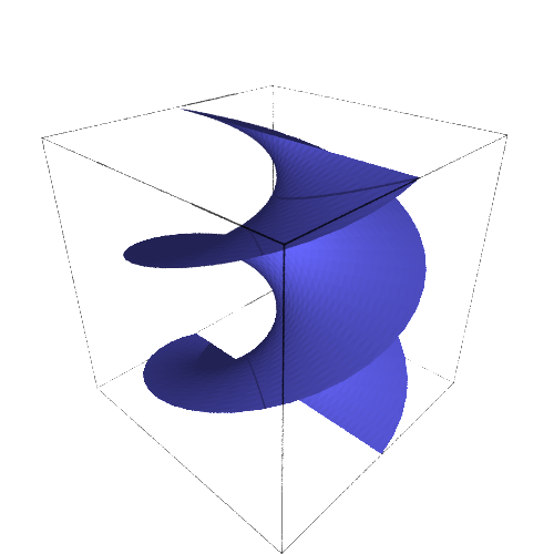
helicoid

Helicoid

Solution. \begin{align*}
\varphi_u&=(\cos v,\sin v,0),\ \varphi_v=(-u\sin v,u\cos v,b),\\
\varphi_{uu}&=0,\ \varphi_{uv}=(-\sin v,\cos v,0),\ \varphi_{vv}=(-u\cos v,-u\sin v,0).
\end{align*}
$E$, $F$ and $G$ are calculated to be
$$E=1,\ F=0,\ G=b^2+u^2.$$
$\varphi_u\times\varphi_v=(b\sin v,-b\cos v,u)$, so the unit normal vector field $N$ is given by
$$N=\frac{\varphi_u\times\varphi_v}{\sqrt{EG-F^2}}=\frac{(b\sin v,-b\cos v,u)}{\sqrt{b^2+u^2}}.$$
Next, $\ell, m,n$ are calculated to be
$$\ell=0,\ m=-\frac{b}{\sqrt{b^2+u^2}},\ n=0.$$
Finally we find the Gaußian curvature $K$ and the mean curvature $H$:
\begin{align*}
K&=\frac{\ell n-m^2}{EG-F^2}=-\frac{b^2}{(b^2+u^2)^2},\\
H&=\frac{G\ell+En-2Fm}{2(EG-F^2)}=0.
\end{align*}
Surfaces with $H=0$ are called minimal surfaces.

For further reading on the topic I discussed here, I recommend:

Barrett O’Neil, Elementary Differential Geometry, Academic Press, 1967