Category Archives: Calculus

Tsiolkovsky Rocket Equation

In this note, we derive the so called Tsiolkovsky rocket equation or simply rocket equation. It is given by
\begin{equation}
\label{eq:rocket}
\Delta v=v_e\ln\frac{m_0}{m_f}=I_{\mathrm{sp}}g_0\ln\frac{m_0}{m_f}
\end{equation}
where

  • $\Delta v$ is the maximum change of velocity of the vehicle;
  • $v_e=I_{\mathrm{sp}}g_0$ is the effective exhaust velocity;
  • $g_0=9.8\ \mathrm{m}/\mathrm{s}^2$ is the gravitational acceleration of an object in a vacuum near the surface of the Earth;
  • $m_0$, called wet mass, is the initial mass, including propellant;
  • $m_f$, called dry mass, is the final total mass without propellant.

The equation \eqref{eq:rocket} is named after the Russian scientist Konstantin Eduardovich Tsiolkovsky (September 5, 1857 – September 19, 1935). He is dubbed the father of Russian rocket science. It is also called fuel equation.

By the Newton’s second law of motion, the net external force $\vec{F}$ to the change in linear momentum $\vec{P}$ of the whole system (including rocket and exhaust) is
$$\vec{F}=\frac{d\vec{P}}{dt}=\lim_{\Delta t\to 0}\frac{\Delta\vec{P}}{\Delta t}$$
$\Delta\vec{P}=\vec{P}_2-\vec{P}_1$, where $\vec{P}_1=m\vec{V}$ is the momentum of the rocket at time $t=0$ and $\vec{P}_2=(m-\Delta m)(\vec{V}+\Delta\vec{V})+\Delta m\vec{V}_e$ is the momentum of the rocket and exhausted mass at $t=\Delta t$. Here, with respect to the observer, $\vec{V}$ is the velocity of the rocket at time $t=0$, $\vec{V}$ is the velocity of the rocket at time $t=\Delta t$, $\vec{V}_e$ is the velocity of the mass added to the exhaust and lost by the rocket during tim $\Delta t$, $m$ is the mass of the rocket at time $t=0$, and $m-\Delta m$ is the mass of the rocket at time $t=\Delta t$. The velocity of the exhaust $\vec{V}_e$ in the observer frame is related to the velocity of the exhaust in the rocket $\vec{v}_e$ by $$\vec{v}_e=\vec{V}_e-\vec{V}$$ or $$\vec{V}_e=\vec{V}+\vec{v}_e$$ Now, $\Delta\vec{P}$ can be written as $$\Delta\vec{P}=m\Delta\vec{V}+\vec{v}_e\Delta m-\Delta m\Delta\vec{V}$$ Since $\Delta m\to 0$ as $\Delta t\to 0$, we have \begin{equation}\label{eq:rocket2}\vec{F}=m\frac{d\vec{V}}{dt}+\vec{v}_e\frac{dm}{dt}\end{equation} If there are no external forces, then $\vec{F}=0$ i.e. $\frac{d\vec{P}}{dt}=0$ (conservation of linear momentum). \eqref{eq:rocket2} then becomes the separable differential equation \begin{equation}\label{eq:rocket3}-m\frac{d\vec{V}}{dt}=\vec{v}_e\frac{dm}{dt}\end{equation} Assuming that $\vec{v}_e$ is constant (Tsiolkovsky’s hypothesis) $v_e$, and integrating \eqref{eq:rocket3} we have $$\int_v^{v+\Delta v}dv=-v_e\int_{m_0}^{m_f}\frac{dm}{m}$$
where $v=|\vec{V}|$, $\Delta v=|\Delta\vec{V}|$, $m_0$ is the initial total mass and $m_f$ is the final mass. Finally, evaluating the integral yields the rocket equation \eqref{eq:rocket}.

From \eqref{eq:rocket}, we obtain
\begin{equation}
\label{eq:rocket4}
\frac{m_0-m_f}{m_0}=1-\frac{m_f}{m_0}=1-e^{-\frac{\Delta v}{v_e}}
\end{equation}
The equation \eqref{eq:rocket4} gives rise to the percentage of the initial total mass which has to be propellant. This tells us how efficient the rocket engine is as shown in the following example.

Example. Let us consider an SSTO (Single-Stage-To-Orbit) rocket. (Most rockets we are seeing are two-stage-to-orbit or three-stage-to-orbit ones.) The rocket uses liquid hydrogen/liquid oxygen for its propellant, so specific impulse is about $I_{\mathrm{sp}}=350$ s. The exhaust velocity is then given by $v_e=3.43$ km/s. $\Delta v$ needed to get the rocket to a 322 km high LEO (Low Earth Orbit) is 8 km/s. With these values \eqref{eq:rocket4} is evaluated to be
$$1-e^{-\frac{\Delta v}{v_e}}=0.9$$
This means that 90% of the initial total mass has to be propellant. The remaining 10% is for the engines, the fuel tank, and the payload. The payload would account for only about 1% of the initial total mass. This kind of rocket is obviously very inefficient and expensive.

In the Sci-Fi novella The Wandering Earth by Liu Cixin (there is also a movie of the same title on Netflix), the Sun will soon become a supernova and facing the ultimate cataclysmic extinction event, people on Earth turns their entire planet into a spaceship and attempt to relocate it to Proxima Centauri which is the closest star to the Sun (about 4.2 light-years). This is an extremely bold idea even in Chinese scale. (Well, they built the Great Wall!) Disappointingly though, in here, I showed using the rocket equation that it is not even possible for startship Earth to break away from its orbit around the Sun.
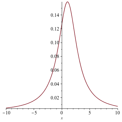
Evaluating $\int\frac{dx}{\sqrt{x^2+a}+b}$

While back, I was calculating a physics problem involving an integral of the form
$$\int\frac{dx}{\sqrt{x^2+a}+b}$$
Naturally, one would begin with the trig substitution $x=a\tan\theta$. So, the integral can be written as
\begin{align*} \int\frac{dx}{\sqrt{x^2+a}+b}&=\int\frac{a\sec^2\theta d\theta}{a\sec\theta+b}\\ &=\frac{1}{a}\int\frac{a^2\sec^2\theta-b^2+b^2}{a\sec\theta+b}d\theta\\ &=\int\sec\theta d\theta-\frac{b}{a}\theta+\frac{b^2}{a}\int\frac{d\theta}{a\sec\theta+b}\\ &=\ln|\sec\theta+\tan\theta|-\frac{b}{\sqrt{b^2-a^2}}\ln\frac{\sqrt{b^2-a^2}\tan\left(\frac{\theta}{2}\right)+a+b}{\sqrt{b^2-a^2}\tan\left(\frac{\theta}{2}\right)-(a+b)}\\ &=\ln\left|\frac{\sqrt{x^2+a^2}+x}{a}\right|-\frac{b}{\sqrt{b^2-a^2}}\ln\left[\frac{\frac{\sqrt{b^2-a^2}x}{a+\sqrt{x^2+a^2}}+a+b}{\frac{\sqrt{b^2-a^2}x}{a+\sqrt{x^2+a^2}}-(a+b)}\right] \end{align*}
Here,
\begin{align*} \int\frac{d\theta}{a\sec\theta+b}&=\int\frac{\cos\theta d\theta}{a+b\cos\theta}\\ &=\frac{1}{b}\int d\theta-\frac{a}{b}\int\frac{d\theta}{a+b\cos\theta}\\ &=\frac{1}{b}\theta-\frac{a}{b}\frac{1}{\sqrt{b^2-a^2}}\ln\frac{\sqrt{b^2-a^2}\tan\left(\frac{\theta}{2}\right)+a+b}{\sqrt{b^2-a^2}\tan\left(\frac{\theta}{2}\right)-(a+b)} \end{align*}
For the evaluation of $\int\frac{d\theta}{a+b\cos\theta}$, I used the formula from here.

The Gaussian Integral

The Gaussian integral is not only important in mathematics but is also extremely important in studying physics, for example, quantum mechanics, quantum field theory, and statistical mechanics. Let us begin with the most simple Gaussian integral
$$G=\int_{-\infty}^\infty e^{-x^2}dx$$
This is not an easy integral to calculate but it can be done easily if we extend it to an integral in two-dimensions as
\begin{align*} G^2&=\int_{-\infty}^\infty e^{-x^2}dx\int_{-\infty}^\infty e^{-y^2}dy\\ &=\int_{-\infty}^\infty\int_{-\infty}^\infty e^{-(x^2+y^2)}dxdy \end{align*}
Now, in term of the polar coordinates, $x=r\cos\theta$, $y=r\sin\theta$ and the area element is $dA=rdrd\theta$, so $G^2$ can be written as
\begin{align*} G^2&=\int_0^{2\pi}\int_0^\infty re^{-r^2}drd\theta\\ &=\pi \end{align*}
The integral $\int_0^\infty re^{-r^2}dr$ can be easily evaluated using the substitution $u=-r^2$ and its value is $\frac{1}{2}$. Now, we obtain
$$G=\int_{-\infty}^\infty e^{-x^2}dx=\sqrt{\pi}$$
From this you can evaluate more complicated Gaussian integrals using a simple substitution and/or some algebra. For example, $\int_{-\infty}^\infty e^{-ax^2}dx$ for a positive real number $a$ can be evaluated easily by a simple substitution $u=\sqrt{a}x$:
\begin{equation}
\begin{aligned}
\int_{-\infty}^\infty e^{-ax^2}dx&=\frac{1}{\sqrt{a}}\int_{-\infty}^\infty e^{-u^2}du\\
&=\sqrt{\frac{\pi}{a}}
\end{aligned}\label{eq:gaussint}
\end{equation}
If $a=\frac{1}{2}$, then $\int_{-\infty}^\infty e^{-\frac{1}{2}x^2}dx=\sqrt{2\pi}$. Normally one will have to use the integration by parts to calculate $\int_{-\infty}^\infty x^2e^{-x^2}dx$ or $\int_{-\infty}^\infty x^4e^{-x^2}dx$. There is a neat trick of evaluating such integrals by differentiating \eqref{eq:gaussint} with respect to $a$:
$$\frac{d}{da}\int_{-\infty}^\infty e^{-ax^2}dx=-\int_{-\infty}^\infty x^2e^{-ax^2}dx$$
and
$$\frac{d}{da}\sqrt{\frac{\pi}{a}}=-\frac{1}{2a}\sqrt{\frac{\pi}{a}}$$
Thus, we have
\begin{equation}
\label{eq:gaussint2}
\int_{-\infty}^\infty x^2e^{-ax^2}dx=\frac{1}{2a}\sqrt{\frac{\pi}{a}}
\end{equation}
For $a=1$, we obtain
$$\int_{-\infty}^\infty x^2e^{-x^2}dx=\frac{\sqrt{\pi}}{2}$$
Differentiating \eqref{eq:gaussint2} with respect to $a$ leads to
\begin{equation}
\label{eq:gaussint3}
\int_{-\infty}^\infty x^4e^{-ax^2}dx=\frac{3}{4a^2}\sqrt{\frac{\pi}{a}}
\end{equation}
For $a=1$, we obtain
\begin{equation}
\label{eq:gaussint4}
\int_{-\infty}^\infty x^4e^{-x^2}dx=\frac{3}{4}\sqrt{\pi}
\end{equation}
I learned this trick from the book Quantum Field Theory in a Nutshell by Anthony Zee. Another important variation is
\begin{equation}
\label{eq:gaussint5}
\int_{-\infty}^\infty e^{-ax^2+bx}dx
\end{equation}
This integral can be evaluated from \eqref{eq:gaussint} with a little bit of algebra. First, by completing the square, we write
\begin{align*} -ax^2+bx&=-a\left(x^2-\frac{b}{a}x\right)\\ &=-a\left(x^2-\frac{b}{a}x+\left(-\frac{b}{2a}\right)^2-\left(-\frac{b}{2a}\right)^2\right)\\ &=-a\left(x-\frac{b}{2a}\right)^2+\frac{b^2}{4a} \end{align*}
Now, \eqref{eq:gaussint5} is evaluated as
\begin{align*} \int_{-\infty}^\infty e^{-ax^2+bx}dx&=\int_{-\infty}^\infty e^{-a\left(x-\frac{b}{2a}\right)^2+\frac{b^2}{4a}}dx\\ &=e^{\frac{b^2}{4a}}\int_{-\infty}^\infty e^{-a\left(x-\frac{b}{2a}\right)^2}dx\\ &=e^{\frac{b^2}{4a}}\int_{-\infty}^\infty e^{-au^2}du\ \left[u=x-\frac{b}{2a}\right]\\ &=e^{\frac{b^2}{4a}}\sqrt{\frac{\pi}{a}} \end{align*}

This time let us try to calculate
\begin{equation}
\label{eq:gaussint6}
\int_{-\infty}^\infty\int_{-\infty}^\infty\int_{-\infty}^\infty (x^2+y^2+z^2)e^{-(x^2+y^2+z^2)}dxdydz
\end{equation}
You stumble upon this type of integral, for example, in a derivation of the Maxwell-Boltzmann statistics in the form of
$$\int d^3p\frac{p^2}{2m}\exp\left(-\beta\frac{p^2}{2m}\right)$$
The integral \eqref{eq:gaussint6} can be easily evaluated using the spherical coordinates:
\begin{align*} x&=r\sin\theta\cos\phi\\ y&=r\sin\theta\sin\phi\\ z&=r\cos\theta\ \end{align*}
where
$$0\leq r<\infty,\ 0\leq\theta\leq\pi,\ 0\leq\theta\leq 2\pi$$
The volume element in the spherical coordinates is $dV=r^2dr\sin\theta d\theta d\phi$, so
\begin{align*} \int_{-\infty}^\infty\int_{-\infty}^\infty\int_{-\infty}^\infty (x^2+y^2+z^2)e^{-(x^2+y^2+z^2)}dxdydz&=\int_0^{2\pi}\int_0^\pi\int_0^\infty r^4e^{-r^2}dr\sin\theta d\theta d\phi\\&=\frac{3}{2}\pi\sqrt{\pi} \end{align*}
We obtain
$$\int_0^\infty r^4e^{-r^2}dr=\frac{3}{8}\sqrt{\pi}$$
using \eqref{eq:gaussint4}.

Evaluating $\int\frac{dx}{a+b\cos x}$ where $b^2>a^2$

One of my Ph.D. students, Victor Zankoni is reading the paper Relativistically corrected Schrödinger equation with Coulomb interaction by J. L. Friar and E. L. Tomusiak, Physical Review C, Volume 29, Number 4, 1537. Following their calculations, he stumbled upon an integral of the form
$$\int\frac{dx}{a+b\cos x}$$
where $b^2>a^2$. Thinking it may not be easy to calculate, I suggested him to look up the well-known book Tables of Integrals, Series, and Products by Gradshteyn and Ryzhik. He said he couldn’t find a relevant formula (actually there is and he somehow missed it) and instead he decided to calculate it. He used a clever substitution and it worked beautifully, so here I am introducing his calculation. First note the identity
$$\cos x=\frac{1-\tan^2\left(\frac{x}{2}\right)}{1+\tan^2\left(\frac{x}{2}\right)}$$
Here, I assume $a>0$ and $b>0$ but similar calculations can be carried out for other cases as well. With the above substitution, we have
\begin{align*} \int\frac{dx}{a+b\cos x}&=\int\frac{\sec^2\left(\frac{x}{2}\right)}{b+a-(b-a)\tan^2\left(\frac{x}{2}\right)}dx\\ &=\frac{2}{b-a}\int\frac{du}{\left(\sqrt{\frac{b+a}{b-a}}\right)^2-u^2}\\ &=\frac{1}{\sqrt{b^2-a^2}}\left[\int\frac{du}{\sqrt{\frac{b+a}{b-a}}+u}+\int\frac{du}{\sqrt{\frac{b+a}{b-a}}-u}\right]\\ &=\frac{1}{\sqrt{b^2-a^2}}\ln\frac{u+\sqrt{\frac{b+a}{b-a}}}{u-\sqrt{\frac{b+a}{b-a}}}\\ &=\frac{1}{\sqrt{b^2-a^2}}\ln\frac{\sqrt{b^2-a^2}u+a+b}{\sqrt{b^2-a^2}u-(a+b)}\\ &=\frac{1}{\sqrt{b^2-a^2}}\ln\frac{\sqrt{b^2-a^2}\tan\left(\frac{x}{2}\right)+a+b}{\sqrt{b^2-a^2}\tan\left(\frac{x}{2}\right)-(a+b)} \end{align*}
The last expression coincides with 2.553 #3 of Gradshteyn and Ryzhik, 8th Edition on page 172. Gradshteyn and Ryzhik 7th Edition does not contain this expression but one can find a supposedly equivalent expression in 2.553 #3 of the 7th Edition but unfortunately, it is stated incorrectly. It has been corrected in the 8th Edition and is listed as 2.553 #4:
$$\int\frac{dx}{a+b\cos x}=\frac{2}{\sqrt{b^2-a^2}}\ln\left|\frac{(b-a)\tan\left(\frac{x}{2}\right)+\sqrt{b^2-a^2}}{(b-a)\tan\left(\frac{x}{2}\right)-\sqrt{b^2-a^2}}\right|\ [b^2>a^2]$$
There is another incorrect formula that caught my eyes:
\begin{align*} \int\frac{dx}{a+b\cos x}&=\frac{2}{\sqrt{b^2-a^2}}\mathrm{arctanh}\left(\frac{(a-b)\tan\left(\frac{x}{2}\right)}{\sqrt{b^2-a^2}}\right)\ \left[b^2>a^2,\ \left|(b-a)\tan\left(\frac{x}{2}\right)\right|<\sqrt{b^2-a^2}\right]\\ &=\frac{2}{\sqrt{b^2-a^2}}\mathrm{arccoth}\left(\frac{(a-b)\tan\left(\frac{x}{2}\right)}{\sqrt{b^2-a^2}}\right)\ \left[b^2>a^2,\ \left|(b-a)\tan\left(\frac{x}{2}\right)\right|>\sqrt{b^2-a^2}\right] \end{align*}
in both 7th Edition and the 8th Edition. It should be corrected to
\begin{align*} \int\frac{dx}{a+b\cos x}&=\frac{2}{\sqrt{b^2-a^2}}\mathrm{arctanh}\left(\frac{(b-a)\tan\left(\frac{x}{2}\right)}{\sqrt{b^2-a^2}}\right)\ \left[b^2>a^2,\ \left|(b-a)\tan\left(\frac{x}{2}\right)\right|<\sqrt{b^2-a^2}\right]\\ &=\frac{2}{\sqrt{b^2-a^2}}\mathrm{arccoth}\left(\frac{(b-a)\tan\left(\frac{x}{2}\right)}{\sqrt{b^2-a^2}}\right)\ \left[b^2>a^2,\ \left|(b-a)\tan\left(\frac{x}{2}\right)\right|>\sqrt{b^2-a^2}\right] \end{align*}
I don’t use Gradshteyn and Ryzhik’s book much but I have heard that it contains numerous typos and mistakes. It appears to be true. So, please use it with caution when you do.

Optimization Problems II: Business and Economic Optimization Problems

In here, we discussed several examples of optimizations problems, mostly geometric optimization problems. In this note, we study business and economic optimization problems. Let us begin with the following example.

Example. Suppose that the price and demand for a particular luxury automobile are related by the demand equation $p+10x=200,000$, where $p$ is the price per car in dollars and $x$ is the number of cars that will be purchased at that price. What price should be charged per car if the total revenue is to be maximized?

Solution. Recall that the total revenue $R$ is given by $R=xp$, where $p$ is the price per item and $x$ is the number of items sold. In terms of $x$, the revenue is written as
$$R(x)=200,000x-10x^2$$
$R(x)=200,000-20x$ and set it equal to 0, we find the critical point $x=10,000$. Since $R^{\prime\prime}(x)=-20<0$, $R(10,000)=100,000,0000$, i.e. a billion dollars. We don’t actually calculus to see this. $R(x)$ is a quadratic function with negative leading coefficient, so it assumes as maximum at the $x$-coordinate of its vertex, $x=-\frac{b}{2a}=-\frac{200,000}{2\cdot 10}=10,000$. To answer the question, the price at which the total revenue $R$ is maximized is
$$p=-10(10,000)+200,000=100,000\ \mathrm{dollars}$$
As you might have noticed by now, it could have been shorter if we wrote $R$ in terms of the price $p$ since the question is about the price at which the revenue is maximized. In terms of $p$, $R$ is written as
$$R(p)=-\frac{p^2}{10}+20,000p$$
Either by solving $R'(p)=-\frac{p}{10}+20,000=0$ or by $p=-\frac{b}{2a}=\frac{20,000}{\frac{2}{10}}$, we find $p=\$ 100,000$.

Example. Suppose that the cost, in dollars, of producing $x$ hundred bicycles is given by $C(x)=x^2-2x+4900$. What is the minimum cost?

Solution. Either by solving $C'(x)=2x-2=0$ or by $x=-\frac{b}{2a}=-\frac{-2}{2\cdot 1}$, we find that $C(x)$ assumes the minimum at $x=1$, i.e. the cost of production is the minimum when 100 bicycles are produced. The minimum cost is $C(1)=4899$ dollars.

Example. In the preceding example, find the minimum average cost.

Solution. Recall that the average cost $\bar C(x)$ is given by $\bar C(x)=\frac{C(x)}{x}$, so we have
$$\bar C(x)=x-2+\frac{4900}{x}$$
Setting $C'(x)=1-\frac{4900}{x^2}$ equal to 0, we find $x=70$. Since $C^{\prime\prime}(x)=\frac{9800}{x^3}>0$ when $x=70$, $\bar C(70)=138$ (in dollars) is the minimum average cost.

Here is an interesting theorem from economics.

Theorem. The average cost is minimized at a level of production at which marginal cost equals average cost, i.e. when
$$C'(x)=\bar C(x)$$

Proof. Since $\bar C(x)=\frac{C(x)}{x}$, we obtain by the quotient rule
$$\bar C'(x)=\frac{xC'(x)-C(x)}{x^2}$$
Setting $\bar C'(x)=0$, we have
$$xC'(x)-C(x)=0,$$
that is
$$C'(x)=\frac{C(x)}{x}=\bar C(x)$$

The preceding example can be quickly answered using this Theorem. Setting $C'(x)=\bar C(x)$, we have
$$2x-2=x-2+\frac{4900}{x}$$
Simplifying this we obtain
$$x^2=4900$$
Hence, $x=70$ as we found earlier.

Example. The cost in dollars of producing $x$ stereos is given by $C(x)=70x+800$. The demand equation is $20p+x=18000$. (a) What level of production maximizes profit? (b) What is the price per stereo when profit is maximized? (c) What is the maximum profit?

Solution. From the demand equation, we obtain $p=-0.05x+900$. Recall that the profit function $P(x)$ is given by
\begin{align*} P(x)&=R(x)-C(x)\\ &=xp-C(x)\\ &=-0.05x^2+900x-(70x+800)\\ &=0.05x^2+830x-800 \end{align*}
Setting $P'(x)=-0.1 x+830$ equal to 0, we find the critical point $x=8300$. $P^{\prime\prime}(x)=-0.1<0$, so the profit has the maximum at $x=8300$.

(a) The level of production that maximizes profit is $x=8300$.

(b) The price per stereo at which profit is maximized is
$$p=-0.05(8300)+900=485\ \mathrm{dollars}$$

(c) The maximum profit is
$$P(8300)=-0.05(8300)^2+830(8300)-800=3,443,700\ \mathrm{dollars}$$

Here is another interesting theorem from economics.

Theorem. The profit is maximized when the marginal revenue equals the marginal cost, that is, when $R'(x)=C'(x)$.

Proof. Differentiating revenue function $P(x)=R(x)-C(x)$, we have
$$P'(x)=R'(x)-C'(x)$$
The critical point is obtained from $P'(x)=0$, i.e. when $R'(x)-C'(x)=0$ or $R'(x)=C'(x)$. That is, when the marginal revenue equals the marginal cost. This completes the proof.

The preceding example can be answered quickly using this theorem. Setting $R'(x)=C'(x)$, we have
$$-0.1x+900=70$$
or
$$x=8300$$

Example. A theater has 204 seats. The manager finds that he can fill all the seats if he charges \$4.00 per ticket. For each ten cents that he raises the ticket price he will sell three fewer seats. What ticket price should he charge to maximize the ticket revenue?

Solution. When the manager increases $n$ cents per ticket price, the number $x(n)$ of tickets sold is $x(n)=204-3n$ and the price $p(n)$ per ticket is $p(n)=4+0.1n$. Then the total revenue is given by
\begin{align*} R(n)&=x(n)p(n)\\ &=(204-3n)(4+0.1n)\\ &=-0.3n^2+8.4n+816 \end{align*}
Setting $R'(n)=-0.6n+8.4$ equal to 0, we find $n=14$. Since $R^{\prime\prime}(n)=-0.6<0$, the ticket revenue is maximized when $n=14$, i.e. when the ticket price is \$4.00+\$1.40=\$5.40.

Alternatively, one can easily find the demand equation which is linear in this case. The equation of line through two points $(204,4)$ and $(201,4.1)$ is given by
$$p=-\frac{1}{30}x+\frac{54}{5}$$
and so we obtain the revenue function
$$R(x)=-\frac{1}{30}x^2+\frac{54}{5}x$$
Setting $R'(x)=-\frac{x}{!5}+\frac{54}{5}$ equal to 0, we find $x=162$ and plugging this into the demand equation for $x$ gives $p=5.40$.

Let us consider a demand equation given as $x=D(p)$. If one were to consider $\frac{dx}{dp}$, the rate of change of demand with respect to price, often it would be convenient to have it as a dimensionless quantity, i.e. one that does not depend on particular units. For that we define a new quantity by dividing $\frac{dx}{dp}$ by $\frac{x}{p}$. The resulting ratio is called the elasticity of demand and is denoted by $\epsilon_D$.

Definition. The elasticity of demand $\epsilon_D$ is defined by
$$\epsilon_D=\frac{\frac{dx}{dp}}{\frac{x}{p}}=\frac{p}{x}\frac{dx}{dp}$$

In economics, demand decreases as price increases, so demand function is a decreasing function, i.e. $\frac{dx}{dp}<0$. Since both $x$ and $p$ are positive, the elasticity $\epsilon_D$ is always negative. The demand is said to be elastic if $|\epsilon_D|>1$, inelastic if $|\epsilon_D|<1$, and unitary if $|\epsilon_D|=1$.

Definition. The relative change of a function whose equation is $p=f(a)$ as $q$ changes from $q_1$ to $q_2$ is
$$\frac{f(q_2)-f(q_1)}{f(q_1)}$$
The percentage change is defined as
$$100\times\frac{f(q_2)-f(q_1)}{f(q_1)}$$

Example. (a) If the demand equation is $x=100-3p$ , find the elasticity of demand when $p=1$.

(b) Show that the elasticity equals the ratio of the relative change in demand to the relative change in price when $p$ changes from 1 to 2.

Solution. (a) $x=100-3p$, $\frac{dx}{dp}=-3$, and when $p=1$, $x=97$, so
$$\epsilon_D=\frac{p}{x}\frac{dx}{dp}=-\frac{3}{97}$$
Since $|\epsilon_D|<1$, the demand is inelastic.

(b) As $p$ changes from 1 to 2, the relative change in price is $\frac{2-1}{1}=1$. When $p$ changes from 1 to 2, $x$ changes from 97 to 94, so the relative change in demand is $-\frac{3}{97}$. Hence, the ration of the relative change in demand to the relative change in price is
$$\frac{-\frac{3}{97}}{1}=-\frac{3}{97}=\epsilon_D$$

Example. Given the demand equation $x=\sqrt{100-2p}$, find the elasticity of demand when $p=18$. Is the demand elastic or inelastic at $p=18$?

Solution. The elasticity $\epsilon_D$ at $p=18$ is
\begin{align*} \epsilon_D&=\frac{p}{x}\frac{dx}{dp}\\ &=\frac{18}{\sqrt{100-2(18)}}\left(-\frac{1}{\sqrt{100-2p}}\right)_{p=18}\\ &=\frac{18}{8}\left(-\frac{1}{8}\right)\\ &=-\frac{9}{32} \end{align*}
Since $|\epsilon_D|=\frac{9}{32}<1$, the demand at $p=18$ is inelastic.

Example. Show that when the revenue is maximized, $|\epsilon_D|=1$.

Solution. The total revenue is $R=xp$, so
\begin{align*} \frac{dR}{dp}&=\frac{dx}{dp}p+x\\ &=x\left(1+\frac{p}{x}\frac{dx}{dp}\right)\\ &=x(1+\epsilon_D) \end{align*}
Since $x>0$, $\frac{dR}{dp}=0$ if and only if $\epsilon_D=-1$. If $\epsilon_D<-1$, then $|\epsilon_D|>1$ i.e. the demand is elastic, and $\frac{dR}{dp}<0$ (the revenue is decreasing). If $-1<\epsilon_D<0$, then $|\epsilon_D|<1$ i.e. the demand is inelastic, and $\frac{dR}{dp}>0$ (the revenue is increasing). So, the revenue is maximized when $|\epsilon_D|=1$.

When demand is a function of price, the elasticity can be written as
$$\epsilon_D=\frac{\frac{p}{x}}{\frac{dp}{dx}}$$