Consider the curve $y=\frac{1}{x}$, $1\leq x<\infty$.

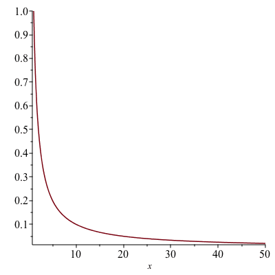
Gabriel’s horn is the surface that is obtained by rotating the above curve about the x-axis.

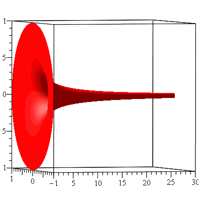
What’s interesting about this Gabriel’s horn is that its surface area is infinite while the volume of its interior is finite. Let us first calculate the volume. Using the disk method, the volume is given by \begin{align*}V&=\pi\int_1^\infty\left(\frac{1}{x}\right)^2dx\\&=\pi\lim_{a\to\infty}\int_1^a\frac{1}{x^2}dx\\&=\pi\lim_{a\to\infty}\left[-\frac{1}{x}\right]_1^a\\&=\pi\lim_{a\to\infty}\left[1-\frac{1}{a}\right]\\&=\pi\end{align*}Its surface area is obtained by calculating the integral \begin{align*}A&=2\pi\int_1^\infty\frac{1}{x}\sqrt{1+\left(-\frac{1}{x^2}\right)^2}dx\\&=2\pi\lim_{a\to\infty}\int_1^a\frac{1}{x}\sqrt{1+\frac{1}{x^4}}dx\end{align*} We don’t actually have to evaluate this integral to see the area is infinite. Since $\sqrt{1+\frac{1}{x^4}}>1$, $$\int_1^a\frac{1}{x}\sqrt{1+\frac{1}{x^4}}dx\geq \int_1^a\frac{1}{x}dx=\ln a$$ Hence, $A=\infty$. The integral $\int \frac{1}{x}\sqrt{1+\frac{1}{x^4}}dx$ can be evaluated exactly. Using first the substitution $u=x^2$ and then the trigonometric substitution $u=\tan\theta$, \begin{align*}\int\frac{1}{x}\sqrt{1+\frac{1}{x^4}}dx&=\frac{1}{2}\int\frac{\sqrt{1+u^2}}{u^2}du\\&=\frac{1}{2}\int\frac{\sec^2\theta\sec\theta}{\tan^2\theta}d\theta\\&=\frac{1}{2}\int\frac{(1+\tan^2\theta)\sec\theta}{\tan^2\theta}d\theta\\&=\frac{1}{2}\left[\int\cot^2\theta\sec\theta d\theta+\int\sec\theta d\theta\right]\\&=\frac{1}{2}\left[\int\frac{\cos\theta}{\sin^2\theta}d\theta+\int\sec\theta d\theta\right]\\&=\frac{1}{2}\left[-\csc\theta+\ln|\sec\theta+\tan\theta|\right]\\&=\frac{1}{2}\left[-\frac{\sqrt{x^4+1}}{x^2}+\ln(\sqrt{x^4+1}+x^2)\right]\end{align*}

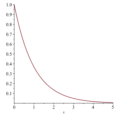
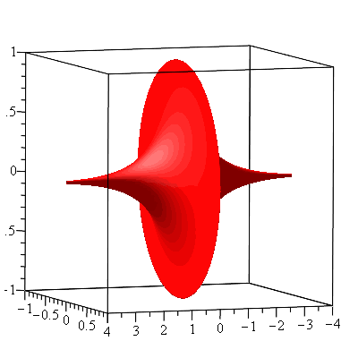
Another horn-shaped surface can be obtained by rotating the curve $y=e^{-x}$, $0\leq x<\infty$:

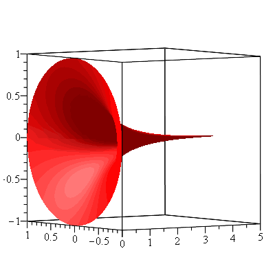
The volume of the interior is finite and \begin{align*}V&=\pi\int_0^\infty e^{-2x}dx\\&=\pi\lim_{a\to\infty}\int_0^\infty e^{-2x}dx\\&=-\frac{\pi}{2}\lim_{a\to\infty}[e^{-2x}]_0^a\\&=\frac{\pi}{2}\end{align*} Unlike Gabriel’s horn, the surface area is also finite. To see that, it is given by the improper integral \begin{align*}A&=\int_0^\infty 2\pi e^{-x}\sqrt{1+(-e^{-x})^2}dx\\&=2\pi\lim_{a\to\infty}\int_0^a e^{-x}\sqrt{1+e^{-2x}}dx\end{align*} Using the substitution $u=e^{-x}$ and then the trigonometric substitution $u=\tan\theta$ the integral $\int e^{-x}\sqrt{1+e^{-2x}}dx$ is evaluated to be \begin{align*}\int e^{-x}\sqrt{1+e^{-2x}}dx&=-\int\sqrt{1+u^2}du\\&=-\int\sec^3\theta d\theta\\&=-\frac{1}{2}[\sec\theta\tan\theta+\ln|\sec\theta+\tan\theta|]\\&=-\frac{1}{2}[u\sqrt{1+u^2}+\ln|\sqrt{u^2+1}+u|]\\&=-\frac{1}{2}[e^{-x}\sqrt{e^{-2x}+1}+\ln(\sqrt{e^{-2x}+1}+e^{-x})]\end{align*} (For the details on how to evaluate the integral $\int\sec^3\theta d\theta$, see here.) Hence, $A$ is computed to be $\pi[\sqrt{2}+\ln(\sqrt{2}+1)]$.

Update: Instead of doing substitutions twice as seen above, one can use a single substitution $e^{-x}=\tan\theta$. The area then turns into the integral $$A=2\pi\int_0^{\frac{\pi}{4}}\sec^3\theta d\theta$$

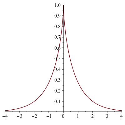
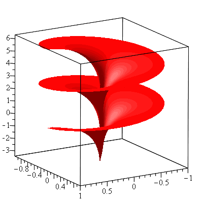
There is a particularly interesting horn-shaped surface (actually a shape of two identical horns put together as shown in the figure below) although it has both a finite volume and a finite surface area. It is called a pseudosphere. A pseudosphere is a surface with constant negative Gaussian curvature. The pseudosphere of radius 1 is obtained by revolving the tractrix $$t\mapsto (t-\tanh t,\mathrm{sech}\ t),\ -\infty<t<\infty$$ about its asymptote (the $x$-axis).

The resulting surface of revolution, the pseudosphere of radius 1, is seen in the following figure.

The volume of the interior of the pseudosphere is \begin{align*}V&=\pi\int_{-\infty}^\infty y^2dx\\&=2\pi\int_0^\infty y^2dx\\&=2\pi\int_0^\infty\mathrm{sech}^2\ t (1-\mathrm{sech}^2\ t)dt\\&=2\pi\int_0^\infty \mathrm{sech}^2\ t\tanh^2 tdt\\&=2\pi\int_0^1 u^2du\ (u=\tanh t)\\&=2\pi\left[\frac{u^3}{3}\right]_0^1\\&=\frac{2\pi}{3}\end{align*} The area of the pseudosphere is \begin{align*}A&=\int_{-\infty}^\infty 2\pi y ds\\&=2\int_0^\infty 2\pi y\sqrt{\left(\frac{dx}{dt}\right)^2+\left(\frac{dy}{dt}\right)^2}dt\\&=4\pi\int_0^\infty\mathrm{sech}\ t\sqrt{(1-\mathrm{sech}^2\ t)^2+(-\mathrm{sech}\ t\tanh t)^2}dt\\&=4\pi\int_0^\infty\mathrm{sech}\ t\sqrt{\tanh^4 t+\mathrm{sech}^2 t\tanh^2 t}dt\\&=4\pi\int_0^\infty\mathrm{sech}\ t\tanh t dt\\&=4\pi\int_0^\infty\frac{\sinh t}{\cosh^2 t}dt\\&=4\pi\int_1^\infty\frac{1}{u^2}du\ (u=\cosh t)\\&=4\pi\end{align*} Notice that its volume is half of the volume of the unit sphere and its area is the same as the area of the unit sphere. Such volume and area relationships are still true for the pseudosphere of radius $r$, i.e. the volume and the area of the pseudosphere of radius $r$ are, respectively, $\frac{2}{3}\pi r^3$ and $4\pi r^2$ (we do not discuss it here, but the radius of a pseudosphere is defined to be the radius of its equator) as noted by the Dutch physicist Christiaan Huygens. The Gaussian curvature of a regular surface can be computed by the Gauss’ formula. The pseudosphere of radius 1 as a parametric surface is represented by the equation $$\varphi(t,s)=(t-\tanh t,\mathrm{sech}\ t\cos s,\mathrm{sech}\ t\sin s)$$ As seen in the figure above, the pseudosphere is not regular along the equator (at $t=0$). It has a constant negative Gaussian curvature $K=-1$ anywhere else. A common misunderstanding (usually by non-mathematicians) is that a surface with constant negative Gaussian curvature is a hyperbolic surface. In order for a surface to be hyperbolic, in addition to having a constant negative curvature, it is required to be complete and regular, so the pseudosphere is not hyperbolic although it was introduced by Eugenio Beltrami as a model of hyperbolic geometry. In fact, Hilbert’s theorem states that there exist no complete regular surface of constant negative Gaussian curvature immersed in $\mathbb{R}^3$. This means that one cannot obtain a model of two-dimensional hyperbolic geometry in $\mathbb{R}^3$. However, one can obtain a model of two-dimensional hyperbolic geoemtry in $\mathbb{R^{2+1}}$, a 3-dimensional Minkowski space-time. There is another interesting surface with constant negative Gaussian curvature called Dini’s surface. It is described by the parametric equations \begin{align*}x&=a\cos u\sin v\\y&=a\sin u\sin v\\z&=a\left(\cos v+\ln\tan\frac{v}{2}\right)+bu\end{align*}

The Gaussian curvature of Dini’s surface is computed to be $K=-\frac{1}{a^2+b^2}$.