Category Archives: Probability

Cauchy Random Variable and Which Improper Integral?

The Cauchy random variable $C(m,a)$ with center $m$ and half-width $a$ is defined by the probability density
$$p(x)=\frac{\frac{a}{\pi}}{(x-m)^2+a^2},\ -\infty\leq x\leq\infty$$

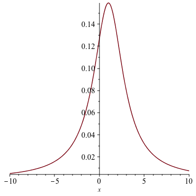
Probability density function $p(x)=\frac{\frac{2}{\pi}}{(x-1)^2+2^2}$.


This $p(x)$ can be considered as a probability density since
\begin{align*}\int_{-\infty}^\infty p(x)dx&=\frac{a}{\pi}\int_{-\infty}^\infty\frac{dx}{(x-m)^2+a^2}\\&=\frac{1}{a\pi}\int_{-\infty}^\infty\frac{du}{\left(\frac{u}{a}\right)^2+1}\ (u=x-m)\\&=\frac{1}{\pi}\int_{-\infty}^\infty\frac{dv}{v^2+1}\ \left(v=\frac{u}{a}\right)\\&=\frac{1}{\pi}\lim_{b\to\infty}\left\{\int_{-b}^0\frac{dv}{v^2+1}+\int_0^b\frac{dv}{v^2+1}\right\}\\&=\frac{1}{\pi}\lim_{b\to\infty}\{[\tan^{-1}(v)]_{-b}^0+[\tan^{-1}(v)]_0^b\}\\&=\frac{1}{\pi}\left\{\frac{\pi}{2}+\frac{\pi}{2}\right\}\\&=1\end{align*}
Now, we want to calculate the mean and obviously, we expect it to be $m$.
\begin{align*}\int_{-\infty}^\infty xp(x)dx&=\frac{a}{\pi}\int_{-\infty}^\infty\frac{x}{(x-m)^2+a^2}dx\\
&=\frac{a}{\pi}\int_{-\infty}^\infty\frac{u}{u^2+a^2}du+\frac{am}{\pi}\int_{-\infty}^\infty\frac{du}{u^2+a^2}\ (u=x-m)\\
&=\frac{a}{\pi}\int_{-\infty}^\infty\frac{u}{u^2+a^2}du+m
\end{align*}
But,
$$\lim_{b\to\infty}\int_{-b}^0\frac{u}{u^2+1}du=\frac{1}{2}\lim_{b\to\infty}[\ln(u^2+a^2)]_{-b}^0=-\infty$$ and $$\lim_{b\to\infty}\int_0^b\frac{u}{u^2+1}du=\frac{1}{2}\lim_{b\to\infty}[\ln(u^2+a^2)]_0^b=\infty$$ This means that the mean does not exist! This result does not coincide with our intuition. What about the Cauchy principal value $$\mathrm{p. v.}\int_{-\infty}^\infty xp(x)dx?$$
Before we continue, recall that if $\int_{-\infty}^\infty f(x)dx$ exists (meaning it is finite) then $\mathrm{p. v.}\int_{-\infty}^\infty f(x)dx$ also exist and
$$\int_{-\infty}^\infty f(x)dx=\mathrm{p. v.}\int_{-\infty}^\infty f(x)dx$$
But the converse need not be true as seen below.
$$\mathrm{p. v.}\int_{-\infty}^\infty f(x)dx=\lim_{b\to\infty}\int_{-b}^b\frac{u}{u^2+1}du=0$$
since $\frac{u}{u^2+1}$ is an odd function. Hence, if we choose to use the Cauchy principal value of the improper integral $\frac{a}{\pi}\int_{-\infty}^\infty\frac{u}{u^2+a^2}du$, we obtain the mean $m$ as expected.

Counting and Combinations: Permutations and Combinatorics

Let us begin with the following example.

Example. In how many ways can 8 horses finish in a race? Here, we assume that there are no ties.

Solution. $8\times 7\times 6\times 5\times 4\times 3\times 2\times 1=40,320$ ways.

The example above shows an ordered arrangement. Such an ordered arrangement is called a permutation.

Definition. $n$ factorial $n!$ is defined by
\begin{align*} n!&=n(n-1)(n-2)\cdots 3\cdot 2\cdot 1,\ n\geq 1\\ 0!&=1 \end{align*}

The number of permutation of $n$ objects is $n!$.

Example. There are $6!$ permutations of the six letters of the word “square”. In how may of them is $r$ the second letter?

Solution. $5\times 1\times 4!=5!=120$.

Example. Five different books are on a shelf. In how many different ways can you arrange them?

Solution. $5!=120$.

We now consider the permutation of a set of objects taken from a larger set. Suppose we have $n$ items. The number of ordered arrangements of $k$ items from the $n$ items can be then found by
$$n(n-1)(n-2)\cdots (n-k+1)=\frac{n!}{(n-k)!}$$
Denote this by ${}_nP_k$.

Example. How many license plates are there that starts with three letters followed by 4 digits (no repetitions)?

Solution. \begin{align*} {}_{26}P_3\times {}_{10}P_4&=\frac{26!}{23!}\times\frac{10!}{6!}\\
&=26\cdot 25\cdot 24\cdot 10\cdot 9\cdot 8\cdot 7\\
&=78,624,000
\end{align*}

Example. How many five-digit zip codes can be made where all digits are different? The possible digits are 0-9.

Solution. ${}_{10}P_5=\frac{10!}{5!}=30,240$.

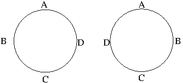
Circular permutations are ordered arrangements of objects in a circle. Suppose that circular permutations such as

are considered as different. Under this assumption, let us consider seating $n$ different objects in a circle. There are $n!$ ways to arrange $n$ seats in a circle depending on where we start and there are $n$ different ways to start seating, so there are $\frac{n!}{n}=(n-1)!$ circular permutations. If the orientation does not matter, i.e. if we consider clockwise and counterclockwise directions are the same, there are $\frac{(n-1)!}{2}$ circular permutations.

Example. In how many ways can you seat 6 persons at a circular dinner table?

Solution. $(6-1)!=5!=120$.

Suppose that we are interested in counting the number of ways to choose $k$ objects from $n$ distinct objects without regard to order. It can be calculated as
$$\frac{{}_nP_k}{k!}=\frac{n!}{k!(n-k)!}$$
This is denoted by ${}_nC_k$ or $\begin{pmatrix}n\\k\end{pmatrix}$ and is read “$n$ choose $k$”.

Example. From a group of 5 women and 7 men, how many different committees consisting of 2 women and 3 men can be formed? What if two of the men are feuding and refuse to serve on the committee together?

Solution. For the first question, there are
\begin{align*} {}_5C_2\times {}_7C_3&=\frac{5!}{2!3!}\times\frac{7!}{3!4!}\\ &=350 \end{align*}
such committees. For the second question, the number of ways to two feuding men and another man is ${}_2C_2\times {}_5C_1=5$. So, the number of selecting male committee members that do not include the two feuding men together is ${}_7C_3-5=30$. Consequently, the number of possible committees in this case is ${}_5C_2\times 30=300$.

Theorem. Suppose that $n$ and $k$ are integers such that $0\leq k\leq n$. Then

  1. ${}_nC_0={}_nC_n=1$ and ${}_nC_1={}_nC_{n-1}=n$.
  2. ${}_nC_k={}_nC_{n-k}$.
  3. Pascal’s identity: ${}_{n+1}C_k={}_nC_{k-1}+{}_nC_k$.

Proof. 2. $${}_nC_{n-k}=\frac{n!}{(n-k)!(n-(n-k))!}=\frac{n!}{(n-k)!k!}={}_nC_k$$

  1. \begin{align*} {}_nC_{k-1}+{}_nC_k&=\frac{n!}{(k-1)!(n-k+1)!}+\frac{n!}{k!(n-k)!}\\ &=\frac{n!k}{k!(n+1-k)!}+\frac{n!(n+1-k)}{k!(n+1-k)!}\\ &=\frac{(n+1)!}{k!(n+1-k)!}\\ &={}_{n+1}C_k
    \end{align*}
    The Pascal’s identity allows us to construct the Pascal’s triangle.
    $$\begin{array}{cccccccccc}
    n & & & & & & & & &\\
    0 & & & & & 1 & & & &\\
    1 & & & & 1 & & 1 & & &\\
    2 & & & 1 & & 2 & & 1 & &\\
    3 & & 1 & & 3 & & 3 & & 1 &\\
    4 & 1 & & 4 & & 6 & & 4 & & 1
    \end{array}$$

Example. The chess club has six members. In how many ways

  1. can all six members line up for a picture?
  2. can they choose a president and a secretary?
  3. can they choose three members to attend a regional tournament with no regard to order?

Solution.

  1. ${}_6P_6=6!=720$.
  2. ${}_6P_2=\frac{6!}{4!}=30$.
  3. ${}_6C_3=\frac{6!}{3!3!}=20$.

Theorem. (Binomial Theorem) Let $n$ be a nonnegative integer. Then
$$(x+y)^n=\sum_{k=0}^n{}_nC_k x^{n-k}y^k$$

Proof. We prove it by induction on $n$. For $n=0$,
$$(x+y)^0=1=\sum_{k=0}^0 {}_0C_k x^{-k}y^k$$ For $n=1$, $$\sum_{k=0}^1 {}_1C_k x^{1-k}y^k=x+y$$ Suppose the statement is true up to $n$, i.e. $$(x+y)^n=\sum_{k=0}^n{}_nC_k x^{n-k}y^k$$ \begin{align*} (x+y)^{n+1}&=(x+y)^n(x+y)\\ &=\sum_{k=0}^n {}_nC_k x^{n-k}y^k\\ &=\sum_{k=0}^n {}_nC_kx^{n+1-k}y^k+\sum_{k=0}^n {}nC_k x^{n-k}y^{k+1}\\ &=\sum_{k=0}^n {}_nC_kx^{n+1-k}y^k+\sum_{k=1}^{n+1} {}_nC{k-1} x^{n+1-k}y^k\ (\mbox{replaing $k$ by $k-1$ in the second sum})\\ &={}_nC_0x^{n+1}+\sum_{k=1}^n[{}_nC_k+{}_nC{k-1}]x^{n+1-k}y^k+{}_nC_n y^{n+1}\\ &={}_{n+1}C_0 x^{n+1}+\sum_{k=1}^n {}_{n+1}C_k x^{n+1-k}y^k+{}_{n+1}C_{n+1} y^{n+1}\ (\mbox{Pascal’s identity})\\
&=\sum_{k=0}^{n+1}{}_{n+1}C_k x^{n+1-k}y^k
\end{align*}
This completes the proof.

Example. Expand $(x+y)^6$ using the Binomial Theorem.

Solution.
$$(x+y)^6=x^6+6x^5y+15x^4y^2+20x^3y^3+15x^2y^4+6xy^5+y^6$$

Example. How many subsets are there of a set with $n$ elements?

Solution. There are ${}nC_k$ subsets of $k$ elements, $0\leq k\leq n$. Hence, the total number of subsets of a set of $n$ elements is $$\sum_{k=0}^n {}_nC_k=(1+1)^n=2^n$$

References:

Marcel B. Finan, A Probability Course for the Actuaries

Sheldon Ross, A First Course in Probability, Fifth Edition, Prentice Hall, 1997

Counting and Combinatorics: The Fundamental Principle of Counting

Example. A lottery allows to select a two-digit number. Each digit may be either 1, 2, or 3. Show all possible out comes. Show all possible outcomes.

Solution. There are three different ways to choose the first digit. For each choice of the first digit, there are three different ways of choosing the second digit (a tree diagram would visually show this). Hence, there are nine possible outcomes of the two-digit numbers and they are
$${11,12,13,21,22,23,31,32,33}$$

Theorem [The Fundamental Principle of Counting]. If a choice consists of $k$ steps, of which the fist can be made in $n_1$ ways, for each of these the second can be made in $n_2$ ways, …, and for each of these the $k$th can be made in $n_k$ ways, then the whole choice can be made in $n_1n_2\cdots n_k$ ways.

Proof. Let $S_i$ denote the set of outcomes for the $i$th task, $i=1,\cdots,k$, and let $n(S_i)=n_i$. Then the set of outcomes for the entire job is
$$S_1\times S_2\times\cdots\times S_k={(s_1,s_2,\cdots,s_k)| s_i\in S_i,\ 1\leq i\leq k}$$
Now, we show that
$$n(S_1\times S_2\times\cdots\times S_k)=n(S_1)n(S_2)\cdots n(S_k)$$
by induction on $k$. Let $k=2$. For each element in $S_1$, there are $n_2$ choices from the set $S_2$ to pair with the element. Thus, $n(S_1\times S_2)=n_1n_2$. Suppose that
$$n(S_1\times S_2\times\cdots\times S_m)=n(S_1)n(S_2)\cdots n(S_m)$$
For each $m$-tuple in $S_1\times S_2\times\cdots\times S_m$, there are $n_{m+1}$ choices of elements in the set $S_{m+1}$ to pair with the $m$-tuple. Thus,
\begin{align*} n(S_1\times S_2\times\cdots\times S_{m+1})&=n(S_1\times S_2\times\cdots\times S_m)n(S_{m+1})\\ &=n(S_1)n(S_2)\cdots n(S_{m+1})\ (\mbox{by the induction hypothesis}) \end{align*}
Therefore, by the induction principle,
$$n(S_1\times S_2\times\cdots\times S_k)=n(S_1)n(S_2)\cdots n(S_k)$$

Example. In designing a study of the effectiveness of migraine medicines, 3 factors were considered.

  1. Medicine (A, B, C, D, Placibo)
  2. Dosage Level (Low, Medium, High)
  3. Dosage Frequency (1, 2, 3, 4 times/day)

In how many possible ways can a migraine patient be given medicine?

Solution. $5\cdot 3\cdot 4=60$ different ways.

Example. How many license-plates with 3 letters followed by 3 digits exist?

Solution. There are $10\cdot 10\cdot 10=1000$ ways to choose 3 digits. For each $3$ digit, there are $26\cdot 26\cdot 26=17,576$ ways to choose 3 letters. Hence, the number of ways to make license-plates is $17,270,576,000$.

Example. How many numbers in the range $1000-9999$ have no repeated digits?

Solution. There are 9 different ways to choose the first digit. For each choice of the first digit, there are 9 different ways to choose the second digit without repeating the first digit. For each choice of the first and the second digits, there are 8 different ways to choose the third digit without repeating the first and the second digits. For each choice of the first, second and third digits, there are 7 different ways to choose the fourth digit without repeating the first, second, third digits repeated. Therefore, the answer is $9\cdot 9\cdot 8\cdot 7=4,536$ ways.

Example. How many license-plates with 3 letters followed by 3 digits if exactly one of the digits is 1.

Solution. \begin{align*} 26\cdot 26\cdot 26\cdot(1\cdot 9\cdot 9+9\cdot 1\cdot 9+9\cdot 9\cdot 1)&=26\cdot 26\cdot 26\cdot 3\cdot 9\cdot 9\\ &=4,270,968 \end{align*}
ways.

References:

  1. Marcel B. Finan, A Probability Course for the Actuaries
  2. Sheldon Ross, A First Course in Probability, Fifth Edition, Prentice Hall, 1997
Independence

Definition. Let $(\Omega,\mathscr{U},P)$ be a probability space. Let $A,B\in\mathscr{U}$ be two events with $P(B)>0$. $P(A|B)$, the probability of $A$ given $B$ is defined by
$$P(A|B)=\frac{P(A\cap B)}{P(B)}\ \mbox{if}\ P(B)>0$$
If the events $A$ and $B$ are independent,
$$P(A)=P(A|B)=\frac{P(A\cap B)}{P(B)}$$
i.e.
$$P(A\cap B)=P(A)P(B)$$
This is true under the assumption that $P(B)>0$ but we take this for the definition even if $P(B)=0$.

Definition. Two events $A$ and $B$ are independent if
$$P(A\cap B)=P(A)P(B)$$

Definition. Let $X_i:\Omega\longrightarrow\mathbb{R}^n$ be random variables, $i=1,\cdots$. Then random variables $X_1,\cdots$ are said to be independent if $\forall$ integers $k\geq 2$ and $\forall$ choices of Borel sets $B_1,\cdots,B_k\subset\mathbb{R}^n$
\begin{align*}
P(X_1\in B_1,X_2\in B_2,&\cdots,X_k\in B_k)=\\
&P(X_1\in B_1)P(X_2\in B_2)\cdots P(X_k\in B_k)
\end{align*}

Theorem. The random variables $X_1,\cdots,X_,m:\Omega\longrightarrow\mathbb{R}^n$ are independent if and only if
\begin{equation}
\label{eq:indepdistrib}
F_{X_1,\cdots,X_m}(x_1,\cdots,x_m)=F_{X_1}(x_1)\cdots F_{X_m}(x_m)
\end{equation}
$\forall x_1\in\mathbb{R}^n$, $\forall i=1,\cdots,m$. If the random variables have densities, \eqref{eq:indepdistrib} is equivalent to
$$f_{X_1,\cdots,X_m}(x_1,\cdots,x_m)=f_{X_1}(x_1)\cdots f_{X_m}(x_m)$$
$\forall x_i\in\mathbb{R}^n$, $\forall i=1,\cdots,m$, where the function $f$ are the appropriate densities.

Proof. Suppose that $X_1,\cdots,X_m$ are independent. Then
\begin{align*}
F_{X_1,\cdots,X_m}(x_1,\cdots,x_m)&=P(X_1\leq x_1,\cdots, X_m\leq x_m)\\
&=P(X_1\leq x_1)\cdots,P(X_m\leq x_m)\\
&=F_{X_1}(x_1)\cdots F_{X_m}(x_m)
\end{align*}
Let $B_1,B_2,\cdots,B_m\subset\mathbb{R}^n$ be Borel sets. Then
\begin{align*}
P(X_1\in B_1,\cdots,X_m\in B_m)&=\int_{B_1\times\cdots\times B_m}f_{X_1,\cdots,X_m}(x_1,\cdots,x_m)dx_1\cdots x_m\\
&=\left(\int_{B_1}f_{X_1}(x_1)dx_1\right)\cdots\left(\int_{B_m}f_{X_m}(x_m)dx_m\right)\\
&=P(X_1\in B_1)P(X_2\in B_2)\cdots P(X_k\in B_k)
\end{align*}
So, $X_1,\cdots,X_m$ are independent.

Theorem. If $X_1,\cdots,X_m$ are independent real-valued random variables with $E(X_i)<\infty$ ($i=1,\cdots,m$) then $E(X_1\cdots X_m)<\infty$ and
$$E(X_1\cdots X_m)=E(X_1)\cdots E(X_m)$$

Proof.
\begin{align*}
E(X_1\cdots X_m)&=\int_{\mathbb{R}^n}x_1\cdots x_m f_{X_1,\cdots,X_m}(x_1,\cdots,x_m)dx_1\cdots x_m\\
&=\left(\int_{\mathbb{R}}x_1f_{X_1}(x_1)dx_1\right)\cdots\left(\int_{\mathbb{R}}x_mf_{X_m}(x_m)dx_m\right)\\
&=E(X_1)\cdots E(X_m)
\end{align*}

Theorem. If $X_1,\cdots,X_m$ are independent real-valued variables with $V(X_i)<\infty$, $i=1,\cdots,m$ then
$$V(X_1+\cdots+X_m)=V(X_1)+\cdots+V(X_m)$$

Proof. We prove for the case when $m=2$. For general $m$ case the proof follows by induction. Let $m_1=E(X_1)$ and $m_2=E(X_2)$. Then
\begin{align*}
E(X_1+X_2)&=\int_{\Omega}(X_1+X_2)dP\\
&=\int_{\Omega}X_1dP+\int_{\Omega}X_2dP\\
&=E(X_1)+E(X_2)\\
&=m_1+m_2
\end{align*}
\begin{align*}
V(X_1+X_2)&=\int_{\Omega}(X_1+X_2-(m_1+m_2))^2dP\\
&=\int_{\Omega}(X_1-m_1)^2dP+\int_{\Omega}(X_2-m_2)^2dP\\
+2\int_{\Omega}(X_1-m_1)(X_2-m_2)dP\\
&=V(X_1)+V(X_2)+2E[(X_1-m_1)(X_2-m_2)]
\end{align*}
For $X_1,X_2$ being independent, we have $E[(X_1-m_1)(X_2-m_2)]=0$. This completes the proof.

References:

Lawrence C. Evans, An Introduction to Stochastic Differential Equations, Lecture Notes

Distribution Functions

Let $(\Omega,\mathscr{U},P)$ be a probability space and $X:\Omega\longrightarrow\mathbb{R}^n$ a randome variable. We define an ordering between two vectors in $\mathbb{R}^n$ as follows: Let $x=(x_1,\cdots,x_n),y=(y_1,\cdots,y_n)\in\mathbb{R}^n$. Then $x\leq y$ means $x_i\leq y_i$ for $i=i,\cdots,n$.

Definition. The distribution function of $X$ is the function $F_X: \mathbb{R}^n\longrightarrow[0,1]$ defined by
$$F_X(x):=P(X\leq x)$$
for all $x\in\mathbb{R}^n$. If $X_1,\cdots,X_m:\Omega\longrightarrow\mathbb{R}^n$ are random variables, their joint distribution function $F_{X_1,\cdots,X_m}:(\mathbb{R}^n)^m\longrightarrow[0,1]$ is defined by
$$F_{X_1,\cdots,X_m}(x_1,\cdots,x_m):=P(X_1\leq x_1,\cdots,X_m\leq x_m)$$
for all $x_i\in\mathbb{R}^n$ and for all $i=1,\cdots,n$.

Definition. Let $X$ be a random variable, $F=F_X$ its distribution function. If there exists a nonnegative integrable function $f:\mathbb{R}^n\longrightarrow\mathbb{R}$ such that
$$F(x)=F(x_1,\cdots,x_n)=\int_{-\infty}^{x_1}\cdots\int_{-\infty}^{x_n}f(y_1,\cdots,y_n)dy_1\cdots dy_n$$
then $f$ is called the density function for $X$. More generally,
$$P(X\in B)=\int_B f(x)dx$$
for all $B\in\mathscr{B}$ where $\mathscr{B}$ is the Borel $\sigma$-algebra.

Example. If $X:\Omega\longrightarrow\mathbb{R}$ has the density function
$$f(x)=\frac{1}{\sqrt{2\pi\sigma^2}}e^{-\frac{|x-m|^2}{2\sigma^2}},\ x\in\mathbb{R}$$
then we say $X$ has a Gaussian or normal distribution with mean $m$ and variance $\sigma^2$. In this case, we write “$X$ is an $N(m,\sigma^2)$ random variable.”

Example. If $X: \Omega\longrightarrow\mathbb{R}^n$ has the density
$$f(x)=\frac{1}{\sqrt{(2\pi)^n\det C}}e^{-\frac{1}{2}(x-m)C^{-1}(x-m)^t},\ x\in\mathbb{R}^n$$
for some $m\in\mathbb{R}^n$ and some positive definite symmetric matrix $C$, we say that “$X$ has a Gaussian or normal distribution with mean $m$ and covariance matrix $C$.” We write $X$ is an $N(m,C)$ random variable. The covariance matrix is given by
\begin{equation}\label{eq:covmatrix}C=E[(X-E(X))^t(X-E(X))]\end{equation}
where $X=(X_1,\cdots,X_n)$, i.e. each $C$ is the matrix whose $(i,j)$ entry is the covariance
$$C_{ij}=\mathrm{cov}(X_i,X_j)=E[(X_i-E(X_i))(X_j-E(X_j))]=E(X_iX_j)-E(X_i)E(X_j)$$
Clearly $C$ is a symmetric matrix. Recall that for a real-valued random matrix $X$ the variance $\sigma^2$ is given by
$$\sigma^2=V(X)=E[(X-E(X))^2]=E[(X-E(X))\cdot (X-E(X))]$$
So one readily sees that \eqref{eq:covmatrix} is a generalization of variance to higher dimensions. It follows from \eqref{eq:covmatrix} that for a vector $b\in\mathbb{R}^n$,
$$V(Xb^t)=bV(X)b^t$$
Since the variance is nonnegative, we see that the covariance matrix is a positive definite matrix. Since $C$ is symmetric, $PCP^{-1}=D$ where $P$ is an orthogonal matrix and $D$ is a diagonal matrix whose main diagonal contains the eigenvalues of $C$. Recall that for two $n\times n$ matrices $A$ and $B$, $\det(AB)=\det(A)\det(B)$ so we see that $\det(C)=\det(D)$. Since all the eigenvalues of a positive definite matrix are positive, $\det(C)>0$.

Lemma. Let $X:\Omega\longrightarrow\mathbb{R}^n$ be a random variable and assume that its distribution function $F=F_X$ has the density $f$. Suppose $g:\mathbb{R}^n\longrightarrow\mathbb{R}$ and $Y=g(X)$ is integrable. Then
$$E(Y)=\int_{\mathbb{R}^n}g(x)f(x)dx$$

Proof. Suppose first that $g$ is a simple function on $\mathbb{R}^n$.
$$g=\sum_{i=1}^mb_iI_{B_i}\ (B_i\in\mathscr{B})$$
\begin{align*}E(g(X))&=\sum_{i=1}^mb_i\int_{\Omega}I_{B_i}(X)dP\\&=\sum_{i=1}^mb_iP(X\in B_i).\end{align*}
But
\begin{align*}\int_{\mathbb{R}^n}g(x)f(x)dx&=\sum_{i=1}^mb_i\int_{\mathbb{R}^n}I_{B_i}f(x)dx\\&=\sum_{i=1}^nb_i\int_{B_i}f(x)dx\\&=\sum_{i=1}^mb_iP(X\in B_i)\end{align*}
Hence proves the lemma for the case $g$ is a simple function. The rest of the argument extends to general $g$ straightforwardly.

Corollary. If $X:\Omega\longrightarrow\mathbb{R}^n$ is a random variable and its distribution function $F=F_X$ has the density $f$, then
$$V(X)=\int_{\mathbb{R}^n}|x-E(X)|^2f(x)dx$$

Proof. Recall that $V(X)=E(|X-E(X)|^2)$. Define $g:\mathbb{R}^n\longrightarrow\mathbb{R}$ by
$$g(x)=|x-E(X)|^2$$
for all $x\in\mathbb{R}^n$. Then by the Lemma we have
$$V(X)=\int_{\mathbb{R}^n}|x-E(X)|^2f(x)dx$$

Corollary. If $X:\Omega\longrightarrow\mathbb{R}$ is a random variable and its distribution function $F=F_X$ has the density $f$, then $E(X)=\int_{-\infty}^\infty xf(x)dx$ and $V(X)=\int_{-\infty}^\infty |x-E(X)|^2f(x)dx$.

Proof. Trivial from the Lemma by taking $g:\mathbb{R}\longrightarrow\mathbb{R}$ the identity map.

Corollary. If $X:\Omega\longrightarrow\mathbb{R}^n$ is a random variable and its distribution function $F=F_X$ has the density $f$, then
$$E(X_1\cdots X_n)=\int_{\mathbb{R}^n}x_1\cdots x_nf(x)dx$$

Proof. Define $g:\mathbb{R}^n\longrightarrow\mathbb{R}$ by
$$g(x)=x_1\cdots x_n\ \mbox{for all}\ x=(x_1,\cdots,x_n)\in\mathbb{R}^n$$
Then the rest follows by the Lemma.

Example. If $X$ is $N(m,\sigma^2)$ then
\begin{align*}
E(X)&=\frac{1}{\sqrt{2\pi\sigma^2}}\int_{-\infty}^\infty xe^{-\frac{(x-m)^2}{2\sigma^2}}dx\\
&=m\\
V(X)&=\frac{1}{\sqrt{2\pi\sigma^2}}\int_{-\infty}^\infty (x-m)^2e^{-\frac{(x-m)^2}{2\sigma^2}}dx\\
&=\sigma^2
\end{align*}
Therefore, $m$ is the mean and $\sigma^2$ is the variance.
References:

Lawrence C. Evans, An Introduction to Stochastic Differential Equations, Lecture Notes