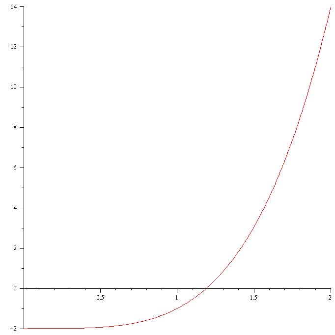
Quadratic equations can be easily solved using the quadratic formula. For cubic and quartic equations there are also formula for solutions, but they are pretty complicated. For polynomials of higher-order degree of 5 or higher there are no such formulas for roots. Newton’s Method allows us to find an approximate solution to such equations. I will use a simple example to explain how it works and then formulate Newton’s method in general. Let us consider the function $f(x)=x^4-2$. Newton’s method begins with by guessing the first solution. In order for Newton’s method to work, one needs to come up with the first guess close enough to the actual solution, otherwise Newton’s method may return an undesirable result. (I will show you an example of such case later on.) We can come up with a reasonable first guess say $x_0$ using the graph of the function.

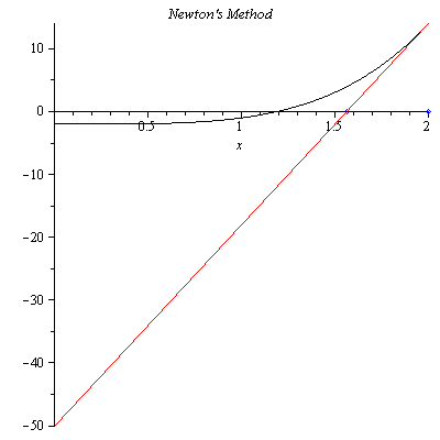
From the graph, we choose $x_0=2$. Of course, one can choose even a closer point, for example $x_0=1.5$. The tangent line to the graph of $f(x)$ at $x_0=2$ is
$$y-f(x_0)=f'(x_0)(x-x_0)$$
Setting $y=0$, we find the $x$-intercept $x_1$
$$x_1=x_0-\frac{f(x_0)}{f'(x_0)}=1.562500000$$

In Figure 2, we see that $x_1$ is closer to the actual solution than $x_0$. This time we find the $x$-intercept $x_2$ of the tangent line to the graph of $f(x)$ at $x_1=1.562500000$.
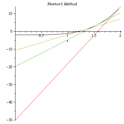
$$x_2=x_1-\frac{f(x_1)}{f'(x_1)}=1.302947000$$

In Figure 3, we see that $x_2$ is closer to the actual solution than $x_1$. Similarly, we can find the next approximate solution $x_3=1.203252569$ which is closer to the actual solution than $x_2$ as shown in Figure 3.

Continuing this process, the 6th approximate solution is given by $x_6=1.189207115$ which is correct to 9 decimal places. The exact solution is $\root 4\of{2}=1.189207115002721$.

In general, Newton’s Method is given by
\begin{align*}x_0&=\mbox{initial approximate}\\x_{n+1}&=x_n-\frac{f(x_n)}{f'(x_n)}\end{align*}
for $n=0,1,2,\cdots$. Here, the assumption is that $f'(x_n)\ne 0$ for $n=0,1,2,\cdots$.

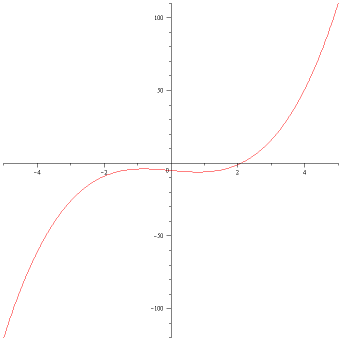
Earlier, I mentioned that if we don’t choose the initial approximate $x_0$ close enough to the actual solution, Newton’s method may return an undesirable result. Let me show you an example. Let us consider the function $f(x)=x^3-2x-5$. Figure 4 shows its graph.

If we choose $x_0=-4$ and run Newton’s method, we obtain the following approximates.

                  X[1] = -2.673913043
                  X[2] = -1.708838801
                  X[3] = -0.7366532045
                  X[4] = -11.29086856
                  X[5] = -7.553673519
                  X[6] = -5.065760748
                  X[7] = -3.400569565
                  X[8] = -2.252794796
                  X[9] = -1.350919123
                 X[10] = 0.01991182580
                 X[11] = -2.501495587
                 X[12] = -1.568413258
                 X[13] = -0.5049189040

As we can see, the numbers do not not appear to be converging to somewhere which indicates that Newton’s method is not working well for this case. In certain cases when we choose $x_0$ too far from the actual solution, we may end up getting $f'(x_n)=0$ for some $n$ in which case Newton’s method fails. For $x_0=4$, we obtain

                   X[1] = 2.891304348
                   X[2] = 2.311222795
                   X[3] = 2.117035157
                   X[4] = 2.094830999
                   X[5] = 2.094551526

The fifth approximate $x_5=2.094551526$ is correct to 6 decimal places.

Newton’s method is not suitable to be carried out by hand. An open source computer algebra system Maxima has a built-in package mnewton for Newton’s method. If you want to install Maxima on your computer, you can find an instruction here. Let us redo the above example using mnewton with initial approximate $x_0=4$.

(%i1) load(“mnewton”)$
(%i2) mnewton([x^3-2*x-5], [x], [4]);
(%o2) [[x = 2.094551481542326]]

What I find interesting about mnewton is that even if you use an initial approximate that didn’t work out for the standard Newton’s method such as $x_0=-4$ in the above example, it instantly returns the answer. (Try it yourself.)

Newton’s method can be used to calculate internal rate of return (IRR) in finance. It is the discount rate at which net present value (NPV) is equal to zero. NPV is the sum of the present values of all cash flows, or alternatively, NPV can be defined as the difference between the present value of the benefits (cash inflows) and the present value of the costs (cash outflows). Here is an example.

Example. If we invest \$100 today and receive \$110 in one year, then NPV can be expressed as
$$\mathrm{NPV}=-100+\frac{110}{1+\mathrm{IRR}}$$
Setting $\mathrm{NPV}=0$, we have
$$\mathrm{IRR}=\frac{110}{100}-1=0.1=10\%$$
If we have multiple future cash inflows \$90, \$50, and \$30 at the end of each year for the next three years, NPV is given by
$$\mathrm{NPV}=-100+\frac{90}{1+\mathrm{IRR}}+\frac{50}{(1+\mathrm{IRR})^2}+\frac{30}{(1+\mathrm{IRR})^3}$$
Setting $\mathrm{NPV}=0$, we obtain a cubic equation
$$100x^3-90x^2-50x-30=0$$
where $x=1+\mathrm{IRR}$. Using Newton’s method, we find $x=1.41$, so $\mathrm{IRR}=0.41=41\%$.

(%i1) load(“mnewton”)$
(%i2) mnewton([100x^3-90x^2-50*x-30], [x], [1]);
(%o2) [[x = 1.406937359155343]]

Update: I wrote a simple Maple script that runs Newton’s method. If you have Maplesoft, you are more than welcome to download the Maple worksheet here and use it.