I am a mathematician and a physics buff. I am interested in studying mathematics inspired by theoretical physics as well as theoretical physics itself. Besides, I am also interested in studying theoretical computer science.
Brachistochrone Problem: Find the shape of the curve down which a bead sliding from rest and accelerated by gravity will slip from on point to another in the least time. Here, we do not consider friction.
Due to conservation of energy, we have \begin{equation} \label{eq:energy} \frac{1}{2}mv^2=mgy \end{equation} Solving \eqref{eq:energy} for the speed $v$, we obtain $$v=\sqrt{2gy}$$ The time $T_{PQ}$ for the bead to travel from a point $P$ to $Q$ is \begin{align*}t_{PQ}&=\int_P^Q\frac{ds}{v}\\&=\int_P^Q\frac{\sqrt{dx^2+dy^2}}{\sqrt{2gy}}\\&=\int_P^Q\sqrt{\frac{1+y_x^2}{2gy}} \end{align*} Let $f(y_x,y)=\sqrt{\frac{1+y_x^2}{2gy}}$. The path from $P$ to $Q$ which minimizes $t_{PQ}$ can be found by solving the Euler-Lagrange equation ([1]) \begin{equation} \label{eq:E-L} \frac{\partial f}{\partial y}-\frac{d}{dx}\frac{\partial f}{\partial y_x}=0 \end{equation} It can be easily shown that \eqref{eq:E-L} is equivalent to \begin{equation} \label{eq:E-L2} \frac{\partial f}{\partial x}-\frac{d}{dx}\left(f-y_x\frac{\partial f}{\partial y_x}\right)=0 \end{equation} Since $f$ does not explicitly depend on $x$, $\frac{\partial f}{\partial x}=0$, so from \eqref{eq:E-L2}, this leads to $$f-y_x\frac{\partial f}{\partial y_x}=C$$ for some constant $C$. On the other hand, we have $$f-y_x\frac{\partial f}{\partial y_x}=\frac{1}{\sqrt{2gy(1+y_x^2)}}$$ Hence, we arrive at the differential equation $$\frac{dy}{dx}=\sqrt{\frac{k^2-y}{y}}$$ where $k^2=\frac{1}{2gC^2}$. The differential equation is separable and it can be written as \begin{equation} \label{eq:de} \sqrt{\frac{y}{k^2-y}}dy=dx \end{equation} Let $\sqrt{\frac{y}{k^2-y}}=\tan\frac{\theta}{2}$. Then $$y=k^2\sin^2\frac{\theta}{2}=\frac{1}{2}k^2(1-\cos\theta)$$ The equation \eqref{eq:de} becomes $$k^2\sin^2\frac{\theta}{2}d\theta=dx$$ Integrating both sides with the half-angle formula $\sin^2\frac{\theta}{2}=\frac{1-\cos\theta}{2}$, we obtain $$x=\frac{1}{2}k^2(\theta-\sin\theta)+C_1$$ for some constant $C_1$. With the condition $P(0,0)$, i.e. $x=y=0$ when $\theta=0$, we have $C_1=0$ and so, $$x=\frac{1}{2}k^2(\theta-\sin\theta)$$ Therefore, the curve on which the bead is sliding down in the shortest time is a cycloid given by the parametric equations \begin{align*}x&=\frac{1}{2}k^2(\theta-\sin\theta)\\y&=\frac{1}{2}k^2(1-\cos\theta)\end{align*} In geometry, a cycloid is the curve traced by a point on a circle as it rolls along a straight line without slipping.
Figure 1. Cycloid with $k=1$ and $0\leq\theta\leq 2\pi$.
References:
George Arfken, Mathematical Methods for Physicists, Third Edition, Academic Press, 1985
Suppose that Boris and Natasha are in different locations far away from each other. Their mutual friend Victor prepares a pair of particles and send one each to Boris and Natasha. Boris chooses to perform one of two possible measurements, say $A_0$ and $A_1$, associated with physical properties $P_{A_0}$ and $P_{A_1}$ of the particle he received. Each $A_0$ and $A_1$ has $+1$ or $-1$ for the outcomes of measurement. When Natasha receives one of the particles, she as well chooses to perform one of two possible measurements $B_0$, $B_1$, each of which has outcome $+1$ or $-1$. Let us consider the following quantity of the measurements $A_0$, $A_1$, $B_0$, $B_1$: $$A_0B_0+A_0B_1+A_1B_0-A_1B_1=(A_0+A_1)B_0+(A_0-A_1)B_1$$ Since $A_0=\pm 1$ and $A_1=\pm 1$, either one of $A_0+A_1$ and $A_0-A_1$ is zero and the other is $\pm 2$. If the experiment is repeated over many trials with Victor preparing new pairs of particles, the expected value of all the outcomes satisfies the inequality \begin{equation} \label{eq:bell} \langle A_0B_0+A_0B_1+A_1B_0-A_1B_1\rangle\leq 2 \end{equation} Proof of \eqref{eq:bell}: \begin{align*}\langle A_0B_0+A_0B_1+A_1B_0-A_1B_1\rangle&=\sum_{A_0,A_1,B_0,B_1}p(A_0,A_1,B_0,B_1)(A_0B_0+A_0B_1+A_1B_0-A_1B_1)\\&\leq \sum_{A_0,A_1,B_0,B_1}2p(A_0,A_1,B_0,B_1)\\&=2 \end{align*} The inequality \eqref{eq:bell} is a variant of the Bell inequality called the CHSH inequality. CHSH stands for John Clauser, Michael Horne, Abner Simony and Richard Holt. The derivation of the CHSH inequality \eqref{eq:bell} depends on two assumptions:
The physical properties $P_{A_0}$, $P_{A_1}$, $P_{B_0}$, $P_{B_1}$ have definite values $A_0$, $A_1$, $B_0$, $B_1$ which exist independently of observation or measurement. This is called the assumption of realism.
Boris performing his measurement does not influence the result of Natasha’s measurement. This is called the assumption of locality.
These two assumptions together are known as the assumptions of local realism. Surprisingly this intuitively innocuous inequality can be violated in quantum mechanics. Here is an example. Let $|0\rangle=\begin{pmatrix} 1\\ 0 \end{pmatrix}$ and $|1\rangle=\begin{pmatrix} 0\\ 1 \end{pmatrix}$. Then $|0\rangle$ and $|1\rangle$ are the eigenstates of $$\sigma_z=\begin{pmatrix} 1 & 0\\ 0 & -1 \end{pmatrix}$$ Victor prepares a quantum system of two qubits in the state \begin{align*}|\psi\rangle&=\frac{|0\rangle\otimes |1\rangle-|1\rangle\otimes |0\rangle}{\sqrt{2}}\\ &=\frac{|01\rangle – |10\rangle}{\sqrt{2}} \end{align*} He passes the first qubit to Boris, and the second qubit to Natasha. Boris measures either of the observables $$A_0=\sigma_z,\ A_1=\sigma_x=\begin{pmatrix} 0 & 1\\ 1 & 0 \end{pmatrix}$$ and Natasha measures either of the observables $$B_0=-\frac{\sigma_x+\sigma_z}{\sqrt{2}},\ B_1=\frac{\sigma_x-\sigma_z}{\sqrt{2}}$$ Since the system is in the state $|\psi\rangle$, the average value of $A_0\otimes B_0$ is \begin{align*}\langle A_0\otimes B_0\rangle&=\langle\psi|A_0\otimes B_0|\psi\rangle\\ &=\frac{1}{\sqrt{2}} \end{align*} Similarly, the average values of the other observables ar given by \begin{align*}\langle A_0\otimes B_1\rangle&=\frac{1}{\sqrt{2}},\ \langle A_1\otimes B_0\rangle=\frac{1}{\sqrt{2}},\ \mbox{and}\\ \langle A_1\otimes B_1\rangle&=-\frac{1}{\sqrt{2}} \end{align*} Since the expected value is linear, we have \begin{equation} \begin{aligned} \langle A_0B_0+A_0B_1+A_1B_0-A_1B_1\rangle&=\langle A_0B_0\rangle+\langle A_0B_1\rangle+\langle A_1B_0\rangle-\langle A_1B_1\rangle\\&=2\sqrt{2}\end{aligned}\label{eq:bell2} \end{equation} This means that the Bell inequality \eqref{eq:bell} is violated. Physicists have confirmed the prediction in \eqref{eq:bell2} by experiments using photons. It turns out that the Mother Nature does not obey the Bell inequality. What this means is that one or both of the two assumptions for the derivation of the Bell inequality \eqref{eq:bell} must be incorrect. There is no consensus among physicists which of the two assumptions needs to be dropped. An important lesson we learn from the Bell inequality is that the Mother Nature (Quantum Mechanics) defies our intuitive common sense. This also begs a troubling question. If we cannot rely on our intuition to understand how the universe works, what else can we rely on? One thing is certain. The world is not locally realistic.
References:
Michael A. Nielsen and Isaac L. Chuang, Quantum Computation and Quantum Information, Cambridge University Press, 2004
Quadratic equations can be easily solved using the quadratic formula. For cubic and quartic equations there are also formula for solutions, but they are pretty complicated. For polynomials of higher-order degree of 5 or higher there are no such formulas for roots. Newton’s Method allows us to find an approximate solution to such equations. I will use a simple example to explain how it works and then formulate Newton’s method in general. Let us consider the function $f(x)=x^4-2$. Newton’s method begins with by guessing the first solution. In order for Newton’s method to work, one needs to come up with the first guess close enough to the actual solution, otherwise Newton’s method may return an undesirable result. (I will show you an example of such case later on.) We can come up with a reasonable first guess say $x_0$ using the graph of the function.
Figure 1. The graph of $f(x)=x^4-2$
From the graph, we choose $x_0=2$. Of course, one can choose even a closer point, for example $x_0=1.5$. The tangent line to the graph of $f(x)$ at $x_0=2$ is $$y-f(x_0)=f'(x_0)(x-x_0)$$ Setting $y=0$, we find the $x$-intercept $x_1$ $$x_1=x_0-\frac{f(x_0)}{f'(x_0)}=1.562500000$$
Figure 2. The first iteration of Newton’s method with $x_0=2$.
In Figure 2, we see that $x_1$ is closer to the actual solution than $x_0$. This time we find the $x$-intercept $x_2$ of the tangent line to the graph of $f(x)$ at $x_1=1.562500000$. $$x_2=x_1-\frac{f(x_1)}{f'(x_1)}=1.302947000$$
Figure 3. The second iteration of Newton’s method with $x_1=1.562500000$.
In Figure 3, we see that $x_2$ is closer to the actual solution than $x_1$. Similarly, we can find the next approximate solution $x_3=1.203252569$ which is closer to the actual solution than $x_2$ as shown in Figure 3.
Figure 4. The third iteration of Newton’s method with $x_2=1.302947000$.
Continuing this process, the 6th approximate solution is given by $x_6=1.189207115$ which is correct to 9 decimal places. The exact solution is $\root 4\of{2}=1.189207115002721$.
In general, Newton’s Method is given by \begin{align*}x_0&=\mbox{initial approximate}\\x_{n+1}&=x_n-\frac{f(x_n)}{f'(x_n)}\end{align*} for $n=0,1,2,\cdots$. Here, the assumption is that $f'(x_n)\ne 0$ for $n=0,1,2,\cdots$.
Earlier, I mentioned that if we don’t choose the initial approximate $x_0$ close enough to the actual solution, Newton’s method may return an undesirable result. Let me show you an example. Let us consider the function $f(x)=x^3-2x-5$. Figure 4 shows its graph.
Figure 5. The graph of $f(x)=x^3-2x-5$.
If we choose $x_0=-4$ and run Newton’s method, we obtain the following approximates.
As we can see, the numbers do not not appear to be converging to somewhere which indicates that Newton’s method is not working well for this case. In certain cases when we choose $x_0$ too far from the actual solution, we may end up getting $f'(x_n)=0$ for some $n$ in which case Newton’s method fails. For $x_0=4$, we obtain
The fifth approximate $x_5=2.094551526$ is correct to 6 decimal places.
Newton’s method is not suitable to be carried out by hand. An open source computer algebra system Maxima has a built-in package mnewton for Newton’s method. If you want to install Maxima on your computer, you can find an instruction here. Let us redo the above example using mnewton with initial approximate $x_0=4$.
What I find interesting about mnewton is that even if you use an initial approximate that didn’t work out for the standard Newton’s method such as $x_0=-4$ in the above example, it instantly returns the answer. (Try it yourself.)
Newton’s method can be used to calculate internal rate of return (IRR) in finance. It is the discount rate at which net present value (NPV) is equal to zero. NPV is the sum of the present values of all cash flows, or alternatively, NPV can be defined as the difference between the present value of the benefits (cash inflows) and the present value of the costs (cash outflows). Here is an example.
Example. If we invest \$100 today and receive \$110 in one year, then NPV can be expressed as $$\mathrm{NPV}=-100+\frac{110}{1+\mathrm{IRR}}$$ Setting $\mathrm{NPV}=0$, we have $$\mathrm{IRR}=\frac{110}{100}-1=0.1=10\%$$ If we have multiple future cash inflows \$90, \$50, and \$30 at the end of each year for the next three years, NPV is given by $$\mathrm{NPV}=-100+\frac{90}{1+\mathrm{IRR}}+\frac{50}{(1+\mathrm{IRR})^2}+\frac{30}{(1+\mathrm{IRR})^3}$$ Setting $\mathrm{NPV}=0$, we obtain a cubic equation $$100x^3-90x^2-50x-30=0$$ where $x=1+\mathrm{IRR}$. Using Newton’s method, we find $x=1.41$, so $\mathrm{IRR}=0.41=41\%$.
Update: I wrote a simple Maple script that runs Newton’s method. If you have Maplesoft, you are more than welcome to download the Maple worksheet here and use it.
Consider the curve $y=\frac{1}{x}$, $1\leq x<\infty$.
The Graph of y=1/x, x=1…50
Gabriel’s horn is the surface that is obtained by rotating the above curve about the x-axis.
Gabriel’s horn
What’s interesting about this Gabriel’s horn is that its surface area is infinite while the volume of its interior is finite. Let us first calculate the volume. Using the disk method, the volume is given by \begin{align*}V&=\pi\int_1^\infty\left(\frac{1}{x}\right)^2dx\\&=\pi\lim_{a\to\infty}\int_1^a\frac{1}{x^2}dx\\&=\pi\lim_{a\to\infty}\left[-\frac{1}{x}\right]_1^a\\&=\pi\lim_{a\to\infty}\left[1-\frac{1}{a}\right]\\&=\pi\end{align*}Its surface area is obtained by calculating the integral \begin{align*}A&=2\pi\int_1^\infty\frac{1}{x}\sqrt{1+\left(-\frac{1}{x^2}\right)^2}dx\\&=2\pi\lim_{a\to\infty}\int_1^a\frac{1}{x}\sqrt{1+\frac{1}{x^4}}dx\end{align*} We don’t actually have to evaluate this integral to see the area is infinite. Since $\sqrt{1+\frac{1}{x^4}}>1$, $$\int_1^a\frac{1}{x}\sqrt{1+\frac{1}{x^4}}dx\geq \int_1^a\frac{1}{x}dx=\ln a$$ Hence, $A=\infty$. The integral $\int \frac{1}{x}\sqrt{1+\frac{1}{x^4}}dx$ can be evaluated exactly. Using first the substitution $u=x^2$ and then the trigonometric substitution $u=\tan\theta$, \begin{align*}\int\frac{1}{x}\sqrt{1+\frac{1}{x^4}}dx&=\frac{1}{2}\int\frac{\sqrt{1+u^2}}{u^2}du\\&=\frac{1}{2}\int\frac{\sec^2\theta\sec\theta}{\tan^2\theta}d\theta\\&=\frac{1}{2}\int\frac{(1+\tan^2\theta)\sec\theta}{\tan^2\theta}d\theta\\&=\frac{1}{2}\left[\int\cot^2\theta\sec\theta d\theta+\int\sec\theta d\theta\right]\\&=\frac{1}{2}\left[\int\frac{\cos\theta}{\sin^2\theta}d\theta+\int\sec\theta d\theta\right]\\&=\frac{1}{2}\left[-\csc\theta+\ln|\sec\theta+\tan\theta|\right]\\&=\frac{1}{2}\left[-\frac{\sqrt{x^4+1}}{x^2}+\ln(\sqrt{x^4+1}+x^2)\right]\end{align*}
Another horn-shaped surface can be obtained by rotating the curve $y=e^{-x}$, $0\leq x<\infty$:
The Graph of y=exp(-x), x=0…5
Surface of revolution of y=exp(-x) about the x-axis
The volume of the interior is finite and \begin{align*}V&=\pi\int_0^\infty e^{-2x}dx\\&=\pi\lim_{a\to\infty}\int_0^\infty e^{-2x}dx\\&=-\frac{\pi}{2}\lim_{a\to\infty}[e^{-2x}]_0^a\\&=\frac{\pi}{2}\end{align*} Unlike Gabriel’s horn, the surface area is also finite. To see that, it is given by the improper integral \begin{align*}A&=\int_0^\infty 2\pi e^{-x}\sqrt{1+(-e^{-x})^2}dx\\&=2\pi\lim_{a\to\infty}\int_0^a e^{-x}\sqrt{1+e^{-2x}}dx\end{align*} Using the substitution $u=e^{-x}$ and then the trigonometric substitution $u=\tan\theta$ the integral $\int e^{-x}\sqrt{1+e^{-2x}}dx$ is evaluated to be \begin{align*}\int e^{-x}\sqrt{1+e^{-2x}}dx&=-\int\sqrt{1+u^2}du\\&=-\int\sec^3\theta d\theta\\&=-\frac{1}{2}[\sec\theta\tan\theta+\ln|\sec\theta+\tan\theta|]\\&=-\frac{1}{2}[u\sqrt{1+u^2}+\ln|\sqrt{u^2+1}+u|]\\&=-\frac{1}{2}[e^{-x}\sqrt{e^{-2x}+1}+\ln(\sqrt{e^{-2x}+1}+e^{-x})]\end{align*} (For the details on how to evaluate the integral $\int\sec^3\theta d\theta$, see here.) Hence, $A$ is computed to be $\pi[\sqrt{2}+\ln(\sqrt{2}+1)]$.
Update: Instead of doing substitutions twice as seen above, one can use a single substitution $e^{-x}=\tan\theta$. The area then turns into the integral $$A=2\pi\int_0^{\frac{\pi}{4}}\sec^3\theta d\theta$$
There is a particularly interesting horn-shaped surface (actually a shape of two identical horns put together as shown in the figure below) although it has both a finite volume and a finite surface area. It is called a pseudosphere. A pseudosphere is a surface with constant negative Gaussian curvature. The pseudosphere of radius 1 is obtained by revolving the tractrix $$t\mapsto (t-\tanh t,\mathrm{sech}\ t),\ -\infty<t<\infty$$ about its asymptote (the $x$-axis).
The Tractrix
The resulting surface of revolution, the pseudosphere of radius 1, is seen in the following figure.
The pseudosphere of radius 1
The volume of the interior of the pseudosphere is \begin{align*}V&=\pi\int_{-\infty}^\infty y^2dx\\&=2\pi\int_0^\infty y^2dx\\&=2\pi\int_0^\infty\mathrm{sech}^2\ t (1-\mathrm{sech}^2\ t)dt\\&=2\pi\int_0^\infty \mathrm{sech}^2\ t\tanh^2 tdt\\&=2\pi\int_0^1 u^2du\ (u=\tanh t)\\&=2\pi\left[\frac{u^3}{3}\right]_0^1\\&=\frac{2\pi}{3}\end{align*} The area of the pseudosphere is \begin{align*}A&=\int_{-\infty}^\infty 2\pi y ds\\&=2\int_0^\infty 2\pi y\sqrt{\left(\frac{dx}{dt}\right)^2+\left(\frac{dy}{dt}\right)^2}dt\\&=4\pi\int_0^\infty\mathrm{sech}\ t\sqrt{(1-\mathrm{sech}^2\ t)^2+(-\mathrm{sech}\ t\tanh t)^2}dt\\&=4\pi\int_0^\infty\mathrm{sech}\ t\sqrt{\tanh^4 t+\mathrm{sech}^2 t\tanh^2 t}dt\\&=4\pi\int_0^\infty\mathrm{sech}\ t\tanh t dt\\&=4\pi\int_0^\infty\frac{\sinh t}{\cosh^2 t}dt\\&=4\pi\int_1^\infty\frac{1}{u^2}du\ (u=\cosh t)\\&=4\pi\end{align*} Notice that its volume is half of the volume of the unit sphere and its area is the same as the area of the unit sphere. Such volume and area relationships are still true for the pseudosphere of radius $r$, i.e. the volume and the area of the pseudosphere of radius $r$ are, respectively, $\frac{2}{3}\pi r^3$ and $4\pi r^2$ (we do not discuss it here, but the radius of a pseudosphere is defined to be the radius of its equator) as noted by the Dutch physicist Christiaan Huygens. The Gaussian curvature of a regular surface can be computed by the Gauss’ formula. The pseudosphere of radius 1 as a parametric surface is represented by the equation $$\varphi(t,s)=(t-\tanh t,\mathrm{sech}\ t\cos s,\mathrm{sech}\ t\sin s)$$ As seen in the figure above, the pseudosphere is not regular along the equator (at $t=0$). It has a constant negative Gaussian curvature $K=-1$ anywhere else. A common misunderstanding (usually by non-mathematicians) is that a surface with constant negative Gaussian curvature is a hyperbolic surface. In order for a surface to be hyperbolic, in addition to having a constant negative curvature, it is required to be complete and regular, so the pseudosphere is not hyperbolic although it was introduced by Eugenio Beltrami as a model of hyperbolic geometry. In fact, Hilbert’s theorem states that there exist no complete regular surface of constant negative Gaussian curvature immersed in $\mathbb{R}^3$. This means that one cannot obtain a model of two-dimensional hyperbolic geometry in $\mathbb{R}^3$. However, one can obtain a model of two-dimensional hyperbolic geoemtry in $\mathbb{R^{2+1}}$, a 3-dimensional Minkowski space-time. There is another interesting surface with constant negative Gaussian curvature called Dini’s surface. It is described by the parametric equations \begin{align*}x&=a\cos u\sin v\\y&=a\sin u\sin v\\z&=a\left(\cos v+\ln\tan\frac{v}{2}\right)+bu\end{align*}
Dini’s surface with a=1 and b=1/2.
The Gaussian curvature of Dini’s surface is computed to be $K=-\frac{1}{a^2+b^2}$.
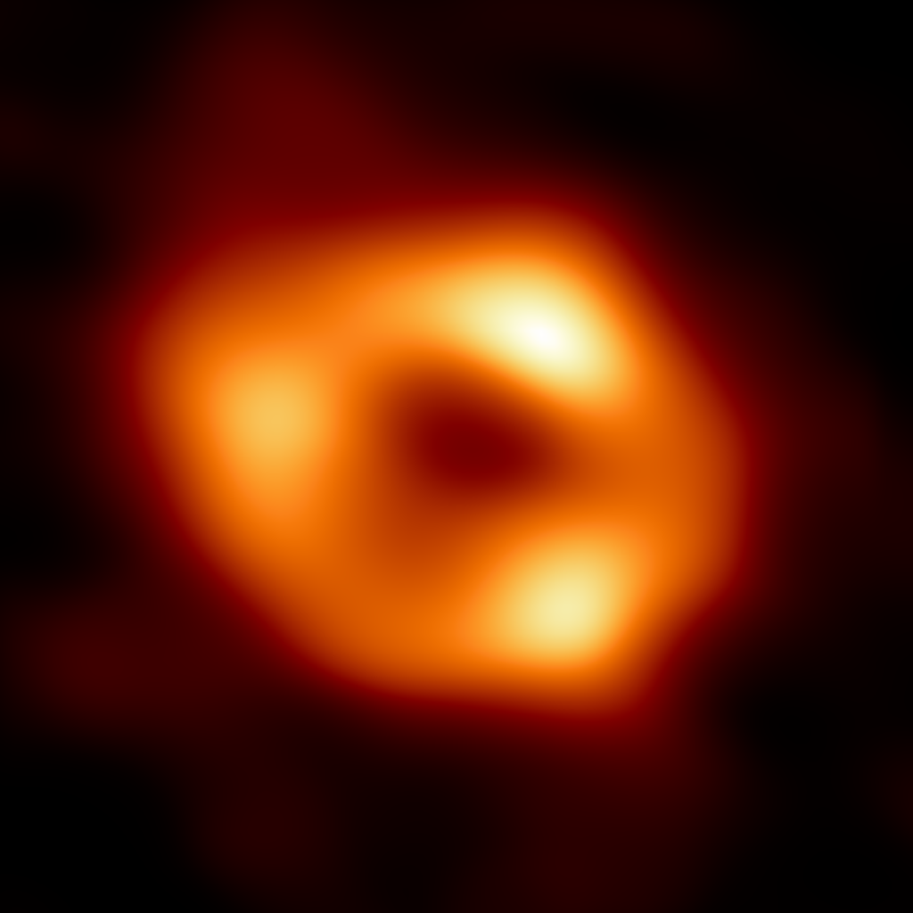
In light of the recent exciting press release about the supermassive black hole at the center of our own Milky Way galaxy, I am going to discuss a brief introduction to black holes and other related concepts in a series of blog articles for those who wish to understand better these amazing monstrous heavenly creatures. For starter, this first article is about Schwarzschild black hole, the simplest black hole model and also the first exact solution of the Einstein’s Field Equation.
The Supermassive Black Hole (Sagittarius A*) at the Center of Milky Way Galaxy.
First, what is a black hole?
A black hole is a hypothetical (though its existence is no longer in doubt) region of spacetime where gravity is so immense that nothing, even light (the lightest matter in the universe) can escape from it.
How did we come to know about a black hole? Was it just an imagination of some mad scientists?
No imagination. We came to know about the theoretical notion of a black hole from Einstein’s general relativity. But long before general relativity came out, French mathematician Pierre-Simon Laplace had already thought about a celestial object whose gravity is so strong that even light can’t escape. It is discussed in his five-volume book Mécanique Céleste (Celestial Mechanics).
In general relativity, black holes are solutions of the Einstein’s Field Equations.
What are the Einstein’s Field Equations?
They are the fundamental equations of Einstein’s theory of gravitation. Such equations are expected to satisfy the following requirements:
The field equations should be independent of coordinate systems, i.e. they should be tensorial.
They should be partial differential equations of second order for the components $g_{ij}$ of the unknown metric tensor. If you want to know what a metric tensor is, go deeper here.
They are a relativistic generalization of the Poisson equation of Newtonian gravitational potential $$\nabla^2\Phi=4\pi G\rho$$ where $\rho$ is the mass density.
Since the energy-momentum tensor $T_{ij}$ is the special relativistic analogue of the mass density, it should be the source of the gravitational field.
If the space is flat, $T_{ij}$ should vanish.
The equations satisfying all these requirements are given by \begin{equation}\label{eq:EFT}G_{ij}=8\pi GT_{ij}\end{equation} where $G_{ij}=R_{ij}-\frac{1}{2}Rg_{ij}$. $G_{ij}$ is called the Einstein tensor. $R_{ij}$ and $R$ are, respectively, Ricci curvature tensor and scalar curvature. If you want to know what they are, go deeper here. Interestingly, the field equations \eqref{eq:EFT} were derived independently and almost simultaneously by Albert Einstein and David Hilbert in 1915.
So, how do we solve the Field Equations?
The field equations are nonlinear partial differential equations. Partial differential equations are, in general, difficult to solve with equations alone. We impose additional (physical) assumptions and conditions (such as boundary conditions and initial conditions) so the equations can becomes simpler enough for us to be able to solve. First, we have no information on the source of gravity, i.e. no information on the energy-momentum tensor $T_{ij}$. Instead, we consider the field equations outside the field-producing masses. Thus, we obtain the vacuum field equations $$R_{ij}-\frac{1}{2}Rg_{ij}=0$$ Without loss of generality, we may assume that the metric tensor $g_{ij}$ is diagonal, i.e. $g_{ij}=0$ if $i\ne j$. This results in $R_{ij}=0$ if $i\ne j$ from the vacuum field equations. For $i=j$, since the scalar curvature $R$ is given by $R=\sum_ig^{ii}R_{ii}$, from the vacuum field equations, we have $(n-2)R=0$. For $n=4$, $R=0$ and therefore the vacuum field equations turn into \begin{equation}\label{eq:ricciflat}R_{ij}=0\end{equation} i.e. vanishing Ricci curvature tensor. \eqref{eq:ricciflat} is simpler than the original vacuum field equations but by no means it is easy to solve. The simplest solution of \eqref{eq:ricciflat} was obtained in 1915 by a German physicist Karl Schwarzschild while serving in the army during World War I. This is also the first exact solution to the Einstein’s field equations. Schwarzschild assumed a static spherical symmetric metric as a solution of the vacuum equations \eqref{eq:ricciflat}. The ansatz for a static isotropic metric is given by \begin{equation}\label{eq:ansatz}ds^2=-A(r)dt^2+B(r)dr^2+r^2(d\theta^2+\sin^2\theta d\phi^2)\end{equation} In addition, we want the solution to become the flat spacetime far away from the masses i.e. the solution is asymptotically flat, so we require $$\lim_{r\to\infty}A(r)=\lim_{r\to\infty}B(r)=1$$ Now, we are ready to solve the vacuum field equations \eqref{eq:ricciflat}. From the ansatz \eqref{eq:ansatz}, we have $$g_{tt}=-A(r),\ g_{rr}=B(r),\ g_{\theta\theta}=r^2,\ g_{\phi\phi}=r^2\sin^2\theta$$ The nonzero Christoffel symbols are computed to be \begin{align*}\Gamma_{rr}^r&=\frac{B’}{2B},\ \Gamma_{tt}^r=\frac{A’}{2B},\ \Gamma_{\theta\theta}^r=-\frac{r}{B}\\\Gamma_{\phi\phi}^r&=-\frac{r\sin^2\theta}{B},\ \Gamma_{\theta r}^\theta=\Gamma_{\phi r}^\phi=\frac{1}{r},\\\Gamma_{tr}^t&=\frac{A’}{2A},\ \Gamma_{\phi\phi}^\theta=-\sin\theta\cos\theta,\ \Gamma_{\phi\theta}^\phi=\cot\theta\end{align*} Here, ‘ stands for $\frac{d}{dr}$. Using these Christoffel symbols, the Ricci tensors are computed to be \begin{align*}R_{tt}&=\frac{A^{\prime\prime}}{2B}-\frac{A’}{4B}\left(\frac{A’}{A}+\frac{B’}{B}\right)+\frac{A’}{rB}\\R_{rr}&=-\frac{A^{\prime\prime}}{2A}+\frac{A’}{4A}\left(\frac{A’}{A}+\frac{B’}{B}\right)+\frac{B’}{rB}\\R_{\theta\theta}&=1-\frac{1}{B}-\frac{r}{2B}\left(\frac{A’}{A}-\frac{B’}{B}\right)\\R_{\phi\phi}&=\sin^2\theta R_{\theta\theta}\end{align*} From the first two equations of the Ricci tensors above and by requirung them to be 0, $$BR_{tt}+AR_{rr}=\frac{1}{rB}(A’B+AB’)=\frac{1}{rB}(AB)’=0$$ So, we have $A(r)B(r)$=constant. Asymptotic flatness implies that $A(r)B(r)=1$. $R_{\theta\theta}=0$ along with $B(r)=\frac{1}{A(r)}$ and $A’B+AB’=0$ results in $A+rA’=(rA)’=1$. Hence, $A(r)=1+\frac{C}{r}$, where $C$ is a constant. By weak field approximation (Newtonian limit) , we obtain \begin{align*}A(r)=-g_{00}&=1+\frac{2\Phi}{c^2}\\&=1-\frac{2MG}{c^2r}\end{align*} where $\Phi=-\frac{GM}{r}$. This determines the constant $C=-\frac{2MG}{c^2r}$. Finally, the Schwarzschild solution is given by \begin{equation}\label{eq:bh}ds^2=-\left(1-\frac{2MG}{c^2r}\right)c^2dt^2+\left(1-\frac{2MG}{c^2r}\right)^{-1}dr^2+r^2(d\theta^2+\sin^2\theta d\phi^2)\end{equation} As I mentioned in the beginning, this is the simplest black hole model and also is the first exact solution of the Einstein’s Field Equations. It turns out that Schwarzschild solution is the only spherically symmetric solution to the vacuum Einstein equation \eqref{eq:ricciflat} due to
Birkhoff’s Theorem
In 1923, George David Birkhoff proved:
Theorem. Any spherically symmetric solution of the vacuum Einstein’s field equations \eqref{eq:ricciflat} must be static and asymptotically flat.
The Shape of a Black Hole
Is the converse of Birkhoff’s theorem true? Namely, is any static and asymptotically flat solution of the vacuum field equations necessarily spherically symmetric? I don’t know the answer, though I assume the answer is known. While the notion of a black hole originated from general relativity as a solution of the field equations, general relativity does not tell us how a black hole can be actually formed. A mechanism of black hole formation was provided by nuclear physics as a consequence of the gravitational collapse of a dead star. From our observations of the shape of massive objects , one would think the shape of a black hole is a sphere also. Since we don’t know (I mean I don’t know) for sure, it would be interesting to ponder whether the shape of a black hole different from a sphere can exist, for example a toroidal (doughnut shaped) black hole. If not for Schwarzschild black hole, how about for a rotational black hole?
Update: Now I know the answers to questions about the converse of Birkhoff’s theorem and the shape of a black hole. I wrote about them here. At the time of writing this article I knew even lesser than what I know now about GR, which is still pretty much close to nothing.
The Event Horizon
I conclude this article by mentioning that the Schwarzschild solution in \eqref{eq:bh} only describes the outside of the black hole. What determines the inside and the outside of a black hole? It is the event horizon. The event horizon is where $r=r_g=\frac{2MG}{c^2}$. $r_g$ is called the Schwarzschild radius.The Schwarzschild solution requires that $r>r_g$. The Schwarzschild solution unfortunately does not tell anything about whatever happens inside the black hole. We will never know for sure what happens once an object falls into a black hole past its event horizon unless we have information on the source of its gravity, i.e. the stress-energy tensor $T_{ij}$.