Related Rates

Related rates problems often involve (context-wise) real-life applications of the chain rule/implicit differentiation. Here are some of the examples that are commonly seen in calculus textbooks.

Example. Car A is traveling west at 50mi/h and car B is traveling north at 60mi/h. Both are headed for the intersection of the two roads. At what rate are the cars approaching each other when car A is 0.3 mi and car B is 0.4 mi from the intersection?

Solution.
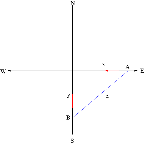
Denote by x and y the distances from the intersection to car A and to car B, respectively. Then we have \frac{dx}{dt}=-50mi/h and \frac{dy}{dt}=-60mi/h. Let us denote z the distance between A and B. Then by Pythagorean law we have z^2=x^2+y^2 Differentiating this with respect to t, we obtain z\frac{dz}{dt}=x\frac{dx}{dt}+y\frac{dy}{dt} and thus \begin{align*}\frac{dz}{dt}&=\frac{1}{z}\left[x\frac{dx}{dt}+y\frac{dy}{dt}\right]\\&=\frac{1}{0.5}[0.3(-50)+0.4(-60)]=-78\mathrm{mi/h}\end{align*}

Example. Air is being pumped into a spherical balloon so that its volume increases at a rate of 100\mathrm{cm}^3/\mathrm{s}. How fast is the radius of the balloon increasing when the diameter is 50 cm?

Solution. Let V and r denote the volume and the radius of the spherical balloon. Then V=\frac{4}{3}\pi r^3. Differentiating this with respect to t, we obtain \frac{dV}{dt}=4\pi r^2\frac{dr}{dt} So, \begin{align*}\frac{dr}{dt}&=\frac{1}{4\pi r^2}\frac{dV}{dt}\\&=\frac{1}{4\pi(25)^2}100\\&=\frac{1}{25\pi}\mathrm{cm/s}\end{align*}

Example. Gravel is being dumped from a conveyor belt at a rate of 30 \mathrm{ft}^3/\mathrm{min} and its coarseness is such that it forms a pile in the shape of a cone whose base diameter and height are the same. How fast is the height of the pile increasing when the pile is 10 ft high?

Solution. The cross section of the gravel pile is shown in the figure below.
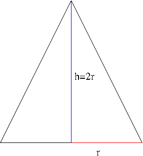
The amount of gravel dumped is the same as the volume of the cone. Let us denote the volume by V, its base radius by r, and its height by h. Then V=\frac{1}{3}\pi r^2h. Since h=2r, V can be written as V=\frac{1}{12}\pi h^3 Differentiating this with respect to t, we obtain \frac{dV}{dt}=\frac{1}{4}\pi h^2\frac{dh}{dt} So, we have \begin{align*}\frac{dh}{dt}&=\frac{4}{\pi h^2}\frac{dV}{dt}\\&=\frac{4}{\pi(10)^2}(30)=\frac{1.2}{\pi}\mathrm{ft/min}\approx 0.38\mathrm{ft/min}\end{align*}

Example. A ladder 10 ft long rests against a vertical wall. If the bottom of the ladder slides away from the wall at a rate of 1 ft/s, how fast is the top of the ladder sliding down the wall when the bottom of the ladder is 6 ft from the wall?

Solution.
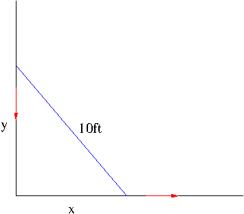
Let us denote by x and y the distance from the wall to the bottom of the ladder and the distance from the top of the ladder to the floor, respectively. By Pythagorean law, we have x^2+y^2=100. Differentiating this with respect to t, we obtain x\frac{dx}{dt}+y\frac{dy}{dt}=0 Hence, we have \begin{align*}\frac{dy}{dt}&=-\frac{x}{y}\frac{dx}{dt}\\&=-\frac{6}{8}(1)=-\frac{3}{4}\mathrm{ft/s}\end{align*}

Example. A water tank has the shape of an inverted circular cone with base radius 2m and heigh 4 m. If water is being pumped into the tank at a rate of 2 \mathrm{m}^3/\mathrm{min}, find the rate at which the water level is rising when the water is 3 m deep.

Solution. The cross section of the water tank is shown in the figure below.
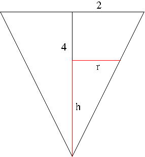
The amount of water V when the water level is h and the surface radius is r is V=\frac{1}{3}\pi r^2h. From the above figure we have the following ratio holds \frac{2}{4}=\frac{r}{h} i.e. r=\frac{h}{2}. SO V can be written as V=\frac{1}{12}\pi h^3 Differentiating this with respect to t, we obtain \frac{dV}{dt}=\frac{1}{4}\pi h^2\frac{dh}{dt} Hence, \begin{align*}\frac{dh}{dt}&=\frac{4}{\pi h^2}\frac{dV}{dt}\\&=\frac{4}{\pi(3)^2}(2)\\&=\frac{8}{9\pi}\mathrm{m/min}\approx 0.28\mathrm{m/min}\end{align*}

Example. A street light is at the top of a 15 feet tall pole. A 6 feet tall woman walks away from the pole with a speed of 5 ft/sec along a straight path. How fast is the tip of her shadow moving when she is 45 feet from the base of the pole?

Solution. Let x be the distance from the light pole to the woman and y be the distance from the light pole to the tip of her shadow as shown in the figure below.
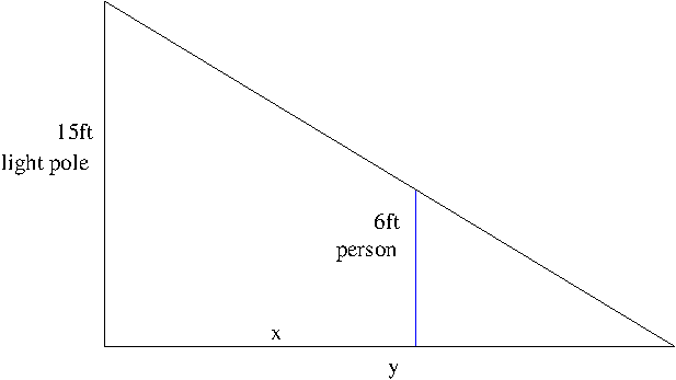
By similar triangles, we have \frac{15}{y}=\frac{6}{y-x}. Solving this equation for y, we obtain y=\frac{5}{3}x. Differentiating this with respect to t, we find how fast the tip of her shadow is moving: \frac{dy}{dt}=\frac{5}{3}\frac{dx}{dt}=\frac{25}{3}\mathrm{ft/s} As seen regardless of how far the woman is from the pole, the speed of the tip is constant.

Example. The fish population, N, in a small pond depends on the amount of algae, a (measured in pounds), in it. The equation modeling the fish population is given by N=(3a^2-20a+26)^4. If the amount of algae is increasing at a rate of 2 lb/week, at what rate is the fish population changing when the pond contains 5 lb of algae?

Solution. By the chain rule, we obtain \begin{align*}\frac{dN}{dt}&=4(3a^2-20a+26)^3\left(6a\frac{da}{dt}-20\frac{da}{dt}\right)\\&=4(3a^2-20a+26)^3(6a-20)\frac{da}{dt}\end{align*} \frac{da}{dt}=2lb/week, so when a=5lb, \frac{dN}{dt} is \frac{dN}{dt}=4(3(5)^2-20(5)+26)^3(6(5)-20)(2)=-80\ \mathrm{lb/week} What this means is that the fish population is decreasing by 80 lb/week at the instant when the pond contains 5 lb of algae.

Example. The retail price per gallon of gasoline is increasing at $0.02 per week. The demand equation is given by 10p-\sqrt{356-x^2}=0 where p is the price per gallon (in dollars), when x million gallons are demanded. At what rate is the revenue changing when 10 million gallons are demanded?

Solution. The total revenue R is given by the equation R=xp Differentiating this equation with respect to t, we obtain \frac{dR}{dt}=\frac{dx}{dt}p+x\frac{dp}{dt} The only quantity we don’t have to calculate \frac{dR}{dt} is \frac{dx}{dt}. To find it, let us differentiate the demand function with respect to x. By the chain rule, we obtain 10\frac{dp}{dt}+\frac{x}{\sqrt{351-x^2}}\frac{dx}{dt}=0 When x=10 million gallons, with \frac{dp}{dt}=0.02, we find from this equation that \frac{dx}{dt}=-0.02\sqrt{256}=-0.02\cdot 16= -0.32\ \mbox{million gallons/week} When x=10, from the demand function, we find p as p=\frac{\sqrt{256}}{10}=\frac{16}{10}=1.6 Therefore, the rate of change of revenue when 10 million gallons of gasoline is demanded is \frac{dR}{dt}=-0.32(1.6)+10(0.02)=-0.312 What this means is that the revenue is decreasing by about 0.31 million dollars per week when the price increases 0.02 dollars per week (consequently the demand decreases by 0.32 million gallons per week as we saw earlier).

Example. A plane flying with a constant speed of 29 km/min passes over a ground radar station at an altitude of 13 km and climbs at an angle of 20 degrees. At what rate is the distance from the plane to the radar station increasing 3 minutes later?

Solution. First, take a look at the following picture
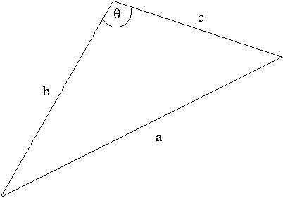
The Law of Cosine

The law of cosine says that the sides a, b, c and the angle \theta are related by a^2=b^2+c^2-2bc\cos\theta

The question above can be pictorially represented as the following sketch
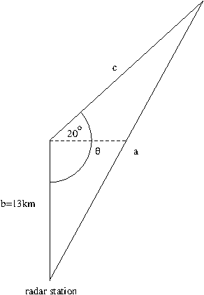
Using the law of cosine with b=13 km, we have a^2=13^2+c^2-2\cdot 13\cdot c\cdot\cos\left(\frac{11}{18}\pi\right) Here, the angle \theta is given by \theta=90^\circ+20^\circ=110^\circ=\frac{11}{18}\pi$ (Note: for this question, you can use degree instead of radian but in that case make sure that your calculator is set to use degree angle measurement.) Since we are to find \frac{da}{dt}, differentiate the above equation with respect to t: 2a\frac{da}{dt}=2c\frac{dc}{dt}-2\cdot 13\frac{dc}{dt}\cos\left(\frac{11}{18}\pi\right) Since the airplane is flying along the side c at the constant speed 29 km/min, it would have traveled c=29\cdot 3=87 km in three minutes. Thus, a=\sqrt{13^2+87^2-2\cdot 13\cdot 87\cos\left(\frac{11}{18}\pi\right)}=92.2586 and hence \frac{da}{dt} in three minutes is \begin{align*}\frac{da}{dt}&=\frac{c}{a}\frac{dc}{dt}-\frac{13}{a}\frac{dc}{dt}\cos\left(\frac{11}{18}\pi\right)\\&=\frac{1}{a}\frac{dc}{dt}\left(c-13\cos\left(\frac{11}{18}\pi\right)\right)\\&=\frac{1}{92.2586}29\left(87-13\cos\left(\frac{11}{18}\pi\right)\right)\\&=28.7447\ \mathrm{km/min}\end{align*}

The Klein-Gordon Equation

For the Schrödinger equation i\hbar\frac{\partial\psi}{\partial t}=\hat H\psi({\bf x},t), the Hamiltonian \hat H=-\frac{\hbar^2}{2m_0}\nabla^2+V({\bf x}) corresponds to the nonrelativistic energy-momentum relation \hat E=\frac{\hat p^2}{2m_0}+V({\bf x}) where \hat E=i\hbar\frac{\partial}{\partial t},\ \hat p=-i\hbar\nabla So, naturally considering the relativistic energy-momentum relation \begin{equation}\label{eq:e-m}\frac{E^2}{c^2}-{\bf p}\cdot{\bf p}=m_0^2c^2\end{equation} would be the starting point to obtain a relativistic generalization of the Schrödinger equation. Replacing E and {\bf p}\cdot{\bf p} in \eqref{eq:e-m} by operators \hat E=i\hbar\frac{\partial}{\partial t}\ \mbox{and}\ \hat p\cdot\hat p=-\hbar^2\nabla^2 acting on a wave function \psi, we obtain the Klein-Gordon equation for a free particle \begin{equation}\label{eq:k-g}\left(\Box-\frac{m_0^2c^2}{\hbar^2}\right)\psi=0\end{equation} where \Box=-\frac{1}{c^2}\frac{\partial^2}{\partial t^2}+\nabla^2

Free solutions of the Schrödinger equation with V({\bf x})=0 are of the form \psi=\exp\left[\frac{i}{\hbar}(-Et+{\bf p}\cdot{\bf x})\right] They are also free solutions of the Klein-Gordon equation \eqref{eq:k-g} with the energy condition E=\pm c\sqrt{m_0^2c^2+p^2} The solutions yielding negative energies appear to be unphysical and initially considered so by physicists, but later they were interpreted as antiparticles. Antiparticles are indeed seen in nature. In reality, antiparticles also have positive energies. Antiparticles as wave functions with negative energies is merely an interpretation of the mathematical representation of the energy condition. If antiparticles weren’t discovered, the negative energy condition would have been still thought to be unphysical.

Other than allowing solutions with negative energies, there was another issue with the Klein-Gordon equation noted by physicists. The conservation of four-current density j_\mu=\frac{i\hbar}{2m_0}(\psi^\ast\nabla_\mu\psi-\psi\nabla_\mu\psi^\ast), where \psi^\ast denotes the complex conjugate of \psi and \nabla_\mu=\left(-\frac{1}{c^2}\frac{\partial}{\partial t},\nabla\right), implies that the quantity \rho=\frac{i\hbar}{2m_0c^2}\left(\psi^\ast\frac{\partial\psi}{\partial t}-\psi\frac{\partial\psi^\ast}{\partial t}\right) can be considered as a probability density. However, the problem is that \rho can be negative. This is due to the appearance of first-order partial derivative \frac{\partial\psi}{\partial t}, which is the consequence of the Klein-Gordon equation being of second-order in time. Because of this, the Klein-Gordon equation was not regarded as a physically viable relativistic generalization of the Schrödinger equation and physicists were instead looking for a relativistic generalization of first-order in time like the Schrödinger equation. Such an equation was finally discovered by P. A. M. Dirac and is called the Dirac equation. On the other hand, the Klein-Gordon equation drew attention of physicists again after they realized that \rho can be interpreted as charge density, and indeed charged pions \pi^+ and \pi^- were discovered. Today, the Klein-Gordon equation is an important relativistic equation that describes charged spin-0 particles.

References:

[1] Walter Greiner, Relativistic Quantum Mechanics, 3rd Edition, Springer-Verlag, 2000

The Curvature

In this note, we study different notions of curvatures of a Riemannian or a pseudo-Riemannian n-manifold M with metric tensor g_{ij}. This note is intended mainly for students of physics. Hence, we will discuss only local expressions of curvatures as those are the ones we mostly use for doing physics in general relativity.

First we need to introduce the Christoffel symbols \Gamma_{ij}^k. The Christoffel symbols are associated with the differentiation of vector fields in a Riemannian or a pseudo Riemannian manifold M, called the Levi-Civita connection. The Levi-Civita connection \nabla is a generalization of the covariant derivative of vector fields in the Euclidean space. Locally the Levi-civita connection is defined by \nabla_{\frac{\partial}{\partial x^i}}\frac{\partial}{\partial x^j}=\sum_{k}\Gamma_{ij}^k\frac{\partial}{\partial x^k} and the Christoffel symbol is given by \Gamma_{ij}^k=\frac{1}{2}\sum_\ell g^{k\ell}\left\{\frac{\partial g_{j\ell}}{\partial x^i}+\frac{\partial g_{\ell i}}{\partial x^j}-\frac{\partial g_{ij}}{\partial x^\ell}\right\} where g^{k\ell} is the inverse of the metric tensor.

Locally the Riemann curvature tensor R_{ijk}^\ell is given by R_{ijk}^\ell=\frac{\partial}{\partial x^j}\Gamma_{ik}^\ell-\frac{\partial}{\partial x^k}\Gamma_{ij}^\ell+\sum_p\left\{\Gamma_{jp}^\ell\Gamma_{ik}^p-\Gamma_{kp}^\ell\Gamma_{ij}^p\right\}

Locally the sectional curvature K(X,Y) of M with respect to the plane spanned by tangent vectors X,Y\in T_pM is given by \begin{equation}\label{eq:sectcurv}K_p(X,Y)=g^{ii}R_{iji}^j\end{equation} assuming that X,Y\in\mathrm{span}\left\{\frac{\partial}{\partial x^i},\frac{\partial}{\partial x^j}\right\}. The sectional curvature is a generalization of the Gaußian curvature of a surface in 3-space. To see this, let \varphi: M^2\longrightarrow M^3 be a conformal parametric surface M^2 immersed in 3-space M^3 with metric e^{u(x,y)}(dx^2+dy^2). The Gaußian curvature K of \varphi can be calculated using the formula (due to Karl Friedrich Gauß) K=\frac{\ell n-m^2}{EG-F^2} where \begin{align*}E&=\langle\varphi_x,\varphi_x\rangle,\ F=\langle\varphi_x,\varphi_y\rangle,\ G=\langle\varphi_y,\varphi_y\rangle,\\\ell&=\langle\varphi_{xx},N\rangle,\ m=\langle\varphi_{xy},N\rangle,\ n=\langle\varphi_{yy},N\rangle\end{align*} Here, \langle\ ,\ \rangle stands for the inner product induced by the conformal metric e^{u(x,y)}(dx^2+dy^2) and N is the unit normal vector field on \varphi. The Gaußian curvature is then obtained as the Liouville’s partial differential equation \begin{equation}\label{eq:liouville}\nabla^2 u=-2Ke^u\end{equation} On the other hand, using \eqref{eq:sectcurv} we find the sectional curvature of \varphi to be g^{11}R_{121}^2=-\frac{e^{u(x,y)}}{2}\nabla^2u which coincides with the Gaußian curvature K from \eqref{eq:liouville}

Example. Let us compute the sectional curvature of the hyperbolic plane \mathbb{H}^2=\{(x,y)\in\mathbb{R}^2: y>0\} with metric ds^2=\frac{dx^2+dy^2}{y^2}

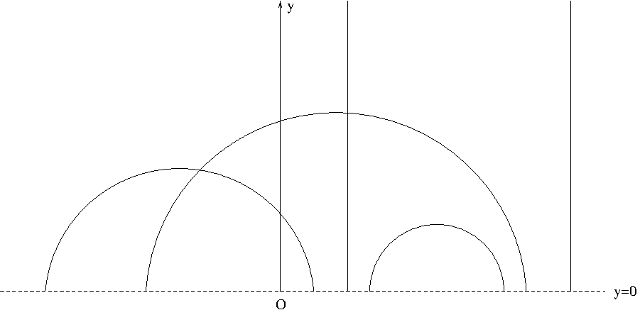
The metric tensor is (g_{ij})=\begin{pmatrix}\frac{1}{y^2} & 0\\0 & \frac{1}{y^2}\end{pmatrix}. The Riemann curvature tensor R_{121}^2 is \begin{align*}R_{121}^2&=\frac{\partial}{\partial y}\Gamma_{11}^2-\frac{\partial}{\partial x}\Gamma_{12}^2+\sum_p\{\Gamma_{2p}^p\Gamma_{11}^p-\Gamma_{1p}^2\Gamma_{12}^p\}\\&=\frac{\partial}{\partial y}\Gamma_{11}^2-\frac{\partial}{\partial x}\Gamma_{12}^2+\Gamma_{21}^2\Gamma_{11}^1-\Gamma_{11}^2\Gamma_{12}^1+\Gamma_{22}^2\Gamma_{11}^2-\Gamma_{12}^2\Gamma_{12}^2\end{align*} We find the Christoffel symbols \Gamma_{11}^2=\frac{1}{y},\ \Gamma_{12}^1=-\frac{1}{y},\ \Gamma_{12}^2=0,\ \Gamma_{21}^2=0,\ \Gamma_{22}^2=-\frac{1}{y} Thus we obtain R_{121}^2=-\frac{1}{y^2} and hence \mathbb{H}^2 has the constant negative sectional curvature K=g^{11}R_{121}^2=y^2\left(-\frac{1}{y^2}\right)=-1 What is the shortest path connecting two points (x_1,y_1) and (x_2,y_2) in \mathbb{H}^2? Such shortest paths are called geodesics in differential geometry. To find out what a geodesic in \mathbb{H}^2 looks like, let J=\int_{(x_1,y_1)}^{(x_2,y_2)}ds=\int_{(x_1,y_1)}^{(x_2,y_2)}\frac{\sqrt{1+y_x^2}}{y}dx where y_x=\frac{dy}{dx}. The shortest path would satisfy the Euler-Lagrange equation \begin{equation}\label{eq:E-L}\frac{\partial f}{\partial x}-\frac{d}{dx}\left(f-y_x\frac{\partial f}{\partial y_x}\right)=0\end{equation}with f(y,y_x,x)=\frac{\sqrt{1+y_x^2}}{y}. Since f does not depend on x, \frac{\partial f}{\partial x}=0 and the Euler-Lagrange equation \eqref{eq:E-L} becomes \frac{d}{dx}\left[\frac{1}{y\sqrt{1+y_x^2}}\right]=0 i.e. \begin{equation}\label{eq:E-L2}\frac{1}{y\sqrt{1+y_x^2}}=C\end{equation} where C is a constant. The equation \eqref{eq:E-L2} results in a separable differential equation \frac{dy}{dx}=\frac{\sqrt{r^2-y^2}}{y} where r^2=\frac{1}{C}. The solution of this equation is (x-a)^2+y^2=r^2 where a is a constant. Since y>0, the solution represents an equation of upper semi circle centered at (a,0) with radius r, that is the shortest path (geodesic) between two points (x_1,y_1) and (x_2,y_2) in \mathbb{H}^2 is a part of an upper semicircle joining them. In particular, if x_1=x_2, the geodesic between (x_1,y_1) and (x_2,y_2) is the vertical line passing through the two points. Such a vertical line can still be considered as an upper semicircle with radius \infty.

Geodesics in Hyperbolic Plane

Two other notions of curvatures are Ricci and scalar curvatures. The Ricci curvature tensor is given by \mathrm{Ric}_p\left(\frac{\partial}{\partial x^i},\frac{\partial}{\partial x^j}\right)=\sum_kR_{ikj}^k We usually denote \mathrm{Ric}_p\left(\frac{\partial}{\partial x^i},\frac{\partial}{\partial x^j}\right) simply by R_{ij}. The scalar curvature \mathrm{Scal}(p) is given by \mathrm{Scal}(p)=\sum_{i}g^{ii}R_{ii} The scalar curvature can be given, in terms of the sectional curvature, by \mathrm{Scal}(p)=\sum_{i\ne j}K_p\left(\frac{\partial}{\partial x^i},\frac{\partial}{\partial x^j}\right) The scalar curvature is usually denoted by R in general relativity.

Definition. A Riemannian or a pseudo-Riemannian manifold (M,g) is said to be maximally symmetric if (M,g) has constant sectional curvature \kappa.

Theorem. If a Riemannian or a pseudo-Riemannian manifold (M,g) is maximally symmetric, then R_{ii}=\kappa(n-1)g_{ii} where \kappa is the constant sectional curvature of (M,g) and n=\dim M.

Corollary. If (M,g) has the constant sectional curvature \kappa, then \mathrm{Scal}(p)=n(n-1)\kappa where n=\dim M.

Riemannian and Pseudo-Riemannian Manifolds

This note is intended particularly for students of physics who have never had any prior encounter with differential geometry. Hence, I try to maintain mathematical rigor and technicalities at a minimum when I discuss differential geometric concepts, instead mostly use hand-waving and rudimentary arguments with emphases on physical ideas and intuition.

The notion of (pseudo-)Riemannian manifolds plays an important role in studying general relativity. But first, what is a manifold? A manifold is, very roughly speaking, a space which locally looks like our space (Euclidean space). In other words, for any point p in a manifold M there exists a neighborhood (called a coordinate neighborhood) U of p such that U\cong\mathbb{R}^n. Here \cong means they are homeomorphic i.e. topologically indistinguishable. Such a property is said to be locally Euclidean and a space which is locally \mathbb{R}^n is called an n-dimensional manifold. Actually being locally Euclidean is not the only condition for a space to be a manifold but that is the most important property of a manifold for physicists.

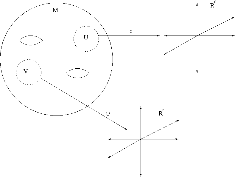
Figure 1, A manifold

Figure 1 shows a manifold M, two coordinate neighborhood U and V with homeomorphisms \phi and \psi, respectively. Why do we need manifolds by the way? In order to do physics, we need coordinates. Without coordinates we can’t write equations of motion. Unfortunately, even for a simple familiar space there is no guarantee that there will be a global coordinate system. Here is an example.

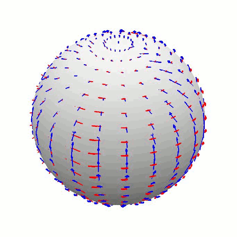
Example. The points (x,y,z) on the 2-sphere S^2 are represented in terms of the spherical coordinates (\theta,\phi) as x=\sin\phi\cos\theta,\ y=\sin\phi\sin\theta,\ z=\cos\phi,\ 0\leq\phi\leq\pi,\ 0\leq\theta\leq 2\pi Using the chain rule, we can write the standard basis \frac{\partial}{\partial\theta}, \frac{\partial}{\partial\phi} for the tangent space T_\ast S^2 in spherical coordinates in terms of the standard basis \frac{\partial}{\partial x}, \frac{\partial}{\partial y}, \frac{\partial}{\partial y} in rectangular coordinates as \begin{align*}\frac{\partial}{\partial\theta}&=-\sin\phi\sin\theta\frac{\partial}{\partial x}+\sin\phi\cos\theta\frac{\partial}{\partial y}\\\frac{\partial}{\partial\phi}&=\cos\phi\cos\theta\frac{\partial}{\partial x}+\cos\phi\sin\theta\frac{\partial}{\partial y}-\sin\phi\frac{\partial}{\partial z}\end{align*} This frame field is not globally defined on S^2 because \frac{\partial}{\partial\theta}=0 at \phi=0,\pi i.e. at the north pole N=(0,0,1) and at the south pole S=(0,0,-1) as also seen in Figure 2.

Figure 2. The 2-sphere with frame field

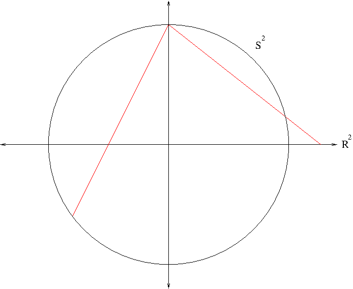
The 2-sphere S^2 is covered by two coordinates neighborhoods U=S^2\setminus{N} and V=S^2\setminus{S}, each of which is identified with \mathbb{R}^2, the Euclidean plane via the stereographic projection. Figure 3 shows the stereographic projection from the north pole N, which is a one-to-one correspondence from U to \mathbb{R}^2.

Figure 3. The Stereographic Projection

A global coordinate system exists in the flat Euclidean space (or a flat pseudo-Euclidean space including Minkowski spacetime), however general relativity has taught us that a physical space is not necessarily a flat space (vaccum spacetime). This is where a manifold comes in. A manifold guarantees the existence coordinate system at least locally and for most cases that is good enough to do physics in particular we write physical equations in a coordinate independent way, so that if a physical equation holds in on coordinate neighborhood, it should also hold in another coordinate neighborhood in the same way.

We would be needing more than topological manifolds to do physics. For an obvious reason we need differentiable manifolds. I am not going to delve into this except for just saying that a differentiable manifold is a manifold on which the differentiability of functions and vector fields can be defined and also to which tangent space at each point can be considered. (If we can’t differentiate fields, we cannot do physics.) In addition, we need Riemannian manifolds. A Riemannian manifold is a differentiable manifold with a Riemannian metric. So what is a Riemannian metric? A Riemannian metric g is a positive definite bilinear symmetric form g_p: T_pM\times T_pM\longrightarrow\mathbb{R}, which induces a positive definite inner product on each tangent space T_pM. In a  coordinate neighborhood, the metric g can be locally given by \begin{equation}\label{eq:metric}g=g_{ij}dx^i\otimes dx^j\end{equation}Here we are using the Einstein’s summation convention. The  n\times n matrix (g_{ij}) is called a metric tensor and physicists often simply write g_{ij} for the metric tensor, not for the component. Since g_{ij} is a symmetric tensor, it can be diagonalized. Since the metric is preserved under diagonalization (which amounts to a change of coordinates), without loss of generality we may assume that g_{ij}=0 if i\ne j so that the metric tensor \eqref{eq:metric} is written as\begin{equation}\label{eq:metric2}g=g_{ii}dx^i\otimes dx^i\end{equation}Let the dimension of M be n. Then each tangent space T_pM is an n-dimensional vector space with the canonical orthonormal basis \left(\frac{\partial}{\partial x^1}\right)_p,\cdots,\left(\frac{\partial}{\partial x^n}\right)_p. Thus any tangent vector v\in T_pM can be written as v=v^j\left(\frac{\partial}{\partial x^j}\right)_p The differential 1-forms d^i are the duals of \frac{\partial}{\partial x^i}, respectively. dx^i\left(\frac{\partial}{\partial x^j}\right)=\delta_{ij} and hence dx^i(v)=v^i For any two tangent vectors v,w\in T_pM using \eqref{eq:metric2} we obtain \begin{equation}\label{eq:metric3}g(v,w)=g_{ii}dx^i\otimes dx^i(v,w)=g_{ii}dx^i(v)dx^i(w)=g_{ii}v^iw^i\end{equation}\eqref{eq:metric3} shows how the metric g induces an inner product on each tangent space T_pM. In doing physics, in particular general relativity, the physical space is often a pseudo-Riemannian manifold rather than a Riemannian manifold. A pseudo-Riemannian manifold is equipped with a pseudo-Riemannian metric which is an indefinite symmetric bilinear form. So the induced inner product is indefinite. A good example is the Minkowski spacetime \mathbb{R}^{3+1} which is \mathbb{R}^4 with the Minkowski metric or the Lorentz-Minkowski metric \begin{equation}\label{eq:minkowski}g=-dt^2+dx^2+dy^2+dz^2\end{equation} The Minkowski metric \eqref{eq:minkowski} induces the inner product on \mathbb{R}^{3+1} (The Minkowski spacetime has a single coordinate neighborhood \mathbb{R}^{3+1} itself and every tangent space T_p\mathbb{R}^{3+1} is isomorphic to \mathbb{R}^{3+1}, hence \mathbb{R}^{3+1} is a manifold and at the same time it is also a vector space.) \langle v,w\rangle=-v^0w^0+v^1w^1+v^2w^2+v^3w^3 where v=(v^0,v^1,v^2,v^3) and w=(w^0,w^1,w^2,w^3) are four-vectors in \mathbb{R}^{3+1}.

In conclusion, I would like to emphasize that the metric tensor g_{ij} is the most important ingredient of a Riemannian or a pseudo-Riemannian manifold. You can literally find out everything about the geometry of a Riemannian or a pseudo-Riemannian manifold with the metric tensor. With the metric tensor, you can also find out about what gravity does when there is matter (the source of gravity) present in the manifold.

Arc Length and Reparametrization

We have already discussed the length of a plane curve represented by the parametric equation {\bf r}(t)=(x(t),y(t)), a\leq t\leq b here. The same goes for a space curve. Namely, if {\bf r}(t)=(x(t),y(t),z(t)), a\leq t\leq b, then its arc length L is given by \begin{equation}\begin{aligned}L&=\int_a^b|{\bf r}'(t)|dt\\&=\int_a^b\sqrt{\left(\frac{dx}{dt}\right)^2+\left(\frac{dy}{dt}\right)^2+\left(\frac{dz}{dt}\right)^2}dt\end{aligned}\label{eq:spacearclength}\end{equation}

Example. Find the length of the arc of the circular helix {\bf r}(t)=\cos t{\bf i}+\sin t{\bf j}+t{\bf k} from the point (1,0,0) to the point (1,0,2\pi).

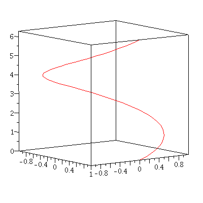
Solution. {\bf r}'(t)=-\sin t{\bf i}+\cos t{\bf j}+{\bf k} so we have |{\bf r}'(t)|=\sqrt{(-\sin t)^2+(\cos t)^2+1^2}=\sqrt{2} The arc is going from (1,0,0) to (1,0,2\pi) and the z-component of {\bf r}(t) is t, so 0\leq t\leq 2\pi. Now, using \eqref{eq:spacearclength}, we obtain L=\int_0^{2\pi}|{\bf r}'(t)|dt=\int_0^{2\pi}\sqrt{2}dt=2\sqrt{2}\pi Figure 1 shows the circular helix from t=0 to t=2\pi.

Figure 1, A circular helix

Given a curve {\bf r}(t), a\leq t\leq b, sometimes we need to reparametrize it by another parameter s for various reasons. Imagine that the curve represents the path of a particle moving in space. A reparametrization does not change the path of the particle (hence nor the distance it traveled) but it changes the particle’s speed! To see this, let t=t(s), \alpha\leq s\leq\beta, a=t(\alpha), b=t(\beta) be an increasing and differentiable function. Since t=t(s) is one-to-one and onto, {\bf r}(t) and {\bf r}(t(s)), its reparametrization by the parameter s, represent the same path. By the chain rule, \begin{equation}\label{eq:reparametrization}\frac{d}{ds}{\bf r}(t(s))=\frac{d}{dt}{\bf r}(t)\frac{dt}{ds}\end{equation} Thus we see that the speed of the reparametrization \left|{\bf r}(t(s))\right| differs from that of {\bf r}(t) by a factor of \left|\frac{dt}{ds}\right|=\frac{dt}{ds} (since \frac{dt}{ds}>0). However, the arc length of the reparametrization is \begin{align*}\int_{\alpha}^{\beta}\left|\frac{d}{ds}{\bf r}(t(s))\right|ds&=\int_{\alpha}^{\beta}\left|\frac{d}{dt}{\bf r}(t)\right|\frac{dt}{ds}ds\\&=\int_a^b\left|\frac{d}{dt}{\bf r}(t)\right|dt=L\end{align*} That is, no change of the distance.

There is a particular reparametrization we are interested. To discuss that, suppose {\bf r}(t), a\leq t\leq b be a differentiable curve in space such that {\bf r}'(t)\ne 0 for all t. Such a curve is said to be regular or smooth. Let us now define the arc length function \begin{equation}\label{eq:arclengthfunction}s(t)=\int_a^t|{\bf r}'(u)|du\end{equation} By the Fundamental Theorem of Calculus, we have \begin{equation}\label{eq:arclengthfunction2}\frac{ds}{dt}=|{\bf r}'(t)|>0\end{equation} and so the arc length function s=s(t) is increasing. This means that s(t) is one-to-one and onto, so it is invertible. It’s inverse function can be written as t=t(s) and {\bf r}(t(s)) is called the reparamerization by arc length. The reason we are interested in this particular reparametrization is that it results in the unit speed: From \eqref{eq:reparametrization} and \eqref{eq:arclengthfunction2}, \left|\frac{d}{ds}{\bf r}(t(s))\right|=|{\bf r}'(t)|\left|\frac{dt}{ds}\right|=|{\bf r}'(t)|\frac{1}{|{\bf r}'(t)|}=1 So it is also called the unit-speed reparametrization. The reparametrization by arc length plays an important role in defining the curvature of a curve. This will be discussed elsewhere.

Example. Reparametrize the helix {\bf r}(t)=\cos t{\bf i}+\sin t{\bf j}+t{\bf k} by arc length measured from (1,0,0)in the direction of increasing t.

Solution. The initial point (1,0,0) corresponds to t=0. From the previous example, we know that the helix has the constant speed |{\bf r}'(t)|=\sqrt{2}. Thus, s(t)=\int_0^t|{\bf r}'(u)|du=\sqrt{2}t Hence, we obtain t=\frac{s}{\sqrt{2}}. The reparametrization is then given by {\bf r}(t(s))=\cos\left(\frac{s}{\sqrt{2}}\right){\bf i}+\sin\left(\frac{s}{\sqrt{2}}\right){\bf j}+\frac{s}{\sqrt{2}}{\bf k}

Examples in this note have been taken from [1].

References.

[1] Calculus, Early Transcendentals, James Stewart, 6th Edition, Thompson Brooks/Cole