
It is very important for students to get familiar with notion of function, some important classes of functions (polynomial functions, rational functions, and trigonometric functions, etc.) and their properties, and trigonometry before they begin to study calculus. If you are not comfortable with any of those I mentioned above, you should brush up as soon as possible.
If you have not studied calculus before, you will notice that it is very different from any subject of mathematics you have encountered before. Calculus deals with a notion of closeness or nearness. Imagine that the variable \(x\) does not just represent a fixed number as a solution of an equation but it keeps changing and approaching a number, say \(2\), closer and closer. This describes a state in which \(x\) is very near the number \(2\). Such a state will be denoted by \(x\to 2\). To get some better picture, you may imagine a flying arrow that keeps getting closer and closer to the target but it never hits the target. Such notion of nearness plays a very important role in mathematics and it is developed into topology, one of the most important and fundamental subjects of mathematics. In particular, the state \(x\to 0\) is called infinitesimal and is also denoted by \(0\). Infinitesimal means “extremely small.” What would be confusing to students who learn calculus for the first time is that infinitesimal \(0\) and the number \(0\) are denoted by the same symbol. There is a branch of advanced mathematics, so-called non-standard analysis. In there, infinitesimal is treated as a number and is denoted by \(0^\ast\) in order to distinguish it from the number \(0\). But we are not going to use this notation. So how do we distinguish them? It turns out that it is not difficult to distinguish them from the context as we will see later. So there is absolutely no reason for you to panic. For the same reason, we often write \(x\to 2\) by \(2\), however it is very important for you to see it, from the context, as a state in which \(x\) is very near 2, not as the fixed number 2. Using the notations from non-standard analysis, it can be written \(2^\ast=2+0^\ast.\) Before we move on, I would like to point out that there are clear distinctions between an infinitesimal \(0\) and the number \(0\). First, an infinitesimal \(0\) can be positive or negative while the number \(0\) is neutral. A positive infinitesimal and a negative infinitesimal may be represented by the notations \(x\to 0+\) and \(x\to 0-\), respectively. The notation \(x\to 0+\) means that \(x\) is approaching \(0\) from the right (or from above \(0\)). Similarly, \(x\to 0-\) means that \(x\) is approaching \(0\) from the left (or from below \(0\)). Second, one can divide a number by an infinitesimal while the division of a number by the number \(0\) is not defined. For instance, \(\frac{1}{0}\) is not defined when \(0\) is a number but \(\frac{1}{0}=\infty\) when \(0\) is a positive infinitesimal. Similarly, \(\frac{1}{0}=-\infty\) if \(0\) is a negative infinitesimal.
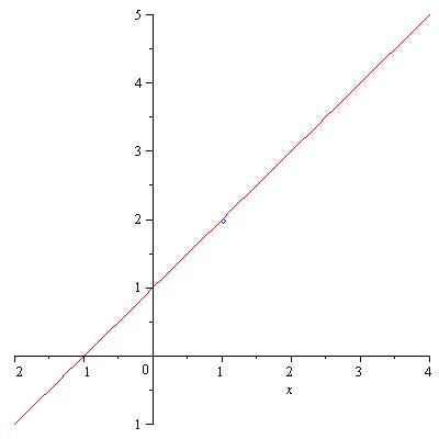
In calculus, we are interested in the behavior of a function near a point. For instance, we want to study how the function \[f(x)=\frac{x^2-1}{x-1}\] behaves near \(x=1\). Note that the function is not defined at \(x=1\). The most direct way to study this is to use sample values of \(x\) that get closer to 1 and see how the values of \(f(x)\) changes.
| Values of \(x\) below and above \(1\) | \(f(x)=\frac{x^2-1}{x-1}\) |
| 0.9 | 1.9 |
| 0.99 | 1.99 |
| 0.999 | 1.999 |
| 0.999999 | 1.999999 |
| 1.1 | 2.1 |
| 1.01 | 2.01 |
| 1.001 | 2.001 |
| 1.0000001 | 2.0000001 |
One can guess from the table that the values of \(f(x)=\frac{x^2-1}{x-1}\) approach \(2\) as both \(x\to 1-\) and \(x\to 1+\). In this case, we say that the limit of \(f(x)=\frac{x^2-1}{x-1}\) is \(2\) as \(x\) approaches \(1\) and write \[\lim_{x\to 1}f(x)=2\] or \[\lim_{x\to 1}\frac{x^2-1}{x-1}=2.\] The following graph of \(f(x)=\frac{x^2-1}{x-1}\) also clearly shows this.
In our example, \[\lim_{x\to 1-}\frac{x^2-1}{x-1}=\lim_{x\to 1+}\frac{x^2-1}{x-1}=2.\] The one-sided limits \(\lim_{x\to a-}f(x)\) and \(\lim_{x\to a+}f(x)\) are called, respectively, the left-hand limit and the right-hand limit of \(f(x)\) at \(x=a\). Clearly we have the following definition.
Definition. We say that the limit \(\lim_{x\to a}f(x)\) exists if both \(\lim_{x\to a-}f(x)\) and \(\lim_{x\to a+}f(x)\) exist and they are the same. The limit \(\lim_{x\to a}f(x)\) is defined to be the value of \(\lim_{x\to a-}f(x)\) (or that of \(\lim_{x\to a+}f(x)\)).
Now we have got some picture of what the limit of a function is. The next important question would be “how do we find the limit?” if it exists. In practice, we do not try to find the limit of a function as we did in the table for reasons. We could only guess the limit by the method and often it can be very difficult to make a guess if the given function is a complicated one. As a result, in many cases you cannot be certain that your guess is correct even if you come up with one. Such method sometimes can easily lead to a wrong answer. If limits exist, there are ways to calculate them exactly. In the above example, again \(x\to 1\) means that \(x\) is very near \(1\) but not exactly equal to \(1\). Since \(x\ne 1\),
\begin{eqnarray*}\lim_{x\to 1}\frac{x^2-1}{x-1}&=&\lim_{x\to 1}\frac{(x+1)(x-1)}{x-1}\\&=&\lim_{x\to 1}(x+1)\\&=&2.\end{eqnarray*}
The method of finding exact values of limits can vary depending on the types of functions. We will discuss more about it later.
Pingback: The Precise Definition of a Limit | MathPhys Archive
Pingback: Limit X 1 X | AllGraphicsOnline.com
Pingback: Calculus 1 Lecture 3: The Precise Definition of a Limit | MathPhys Archive