In this lecture notes, we study basic measure theory in terms of probability. If you want to learn more about general measure theory, I recommend [2].
Let $\Omega$ be a set whose elements will be called samples.
Definition. A $\sigma$-algebra is a collection $\mathscr{U}$ of subsets of $\Omega$ satisfying
- $\varnothing,\Omega\in\mathscr{U}$
- If $A\in\mathscr{U}$, then $A^c\in\mathscr{U}$
- If $A_1,A_2,\cdots\in\mathscr{U}$, then $\bigcup_{k=1}^\infty A_k,\bigcap_{k=1}^\infty A_k\in\mathscr{U}$
Note: In condition 3, it suffices to say if $A_1,A_2,\cdots\in\mathscr{U}$, then $\bigcup_{k=1}^\infty A_k\in\mathscr{U}$ or if $A_1,A_2,\cdots\in\mathscr{U}$, then $\bigcap_{k=1}^\infty A_k\in\mathscr{U}$. For example, lets assume that if $A_1,A_2,\cdots\in\mathscr{U}$, then $\bigcup_{k=1}^\infty A_k\in\mathscr{U}$. Let $A_1,A_2,\cdots\in\mathscr{U}$. Then by condition 2, $(A_1)^c,(A_2)^c,\cdots\in\mathscr{U}$ so we have $\bigcup_{k=1}^\infty (A_k)^c\in\mathscr{U}$. By condition 2 again with De Morgan’s laws, this means $\bigcap_{k=1}^\infty A_k=\left[\bigcup_{k=1}^\infty (A_k)^c\right]^c\in\mathscr{U}$.
Definition. Let $\mathscr{U}$ be a $\sigma$-algebra of subsets of $\Omega$. A map $P:\mathscr{U}\longrightarrow[0,1]$ a probability measure if $P$ satisfies
- $P(\varnothing)=0$, $P(\Omega)=1$
- If $A_1,A_2,\cdots\in\mathscr{U}$, then $$P\left(\bigcup_{k=1}^\infty A_k\right)\leq\sum_{k=1}^\infty P(A_k)$$
- If $A_1,A_2,\cdots\in\mathscr{U}$ are mutually disjoint, then $$P\left(\bigcup_{k=1}^\infty A_k\right)=\sum_{k=1}^\infty P(A_k)$$
Proposition. Let $A,B\in\mathscr{U}$. If $A\subset B$ then $P(A)\leq P(B)$.
Proof. Let $A,B\in\mathscr{U}$ with $A\subset B$. Then $B=(B-A)\dot\cup A$ where $\dot\cup$ denotes disjoint union. So by condition 3, $P(B)=P(B-A)+P(A)\geq P(A)$ since $P(B-A)\geq 0$.
Definition. A triple $(\Omega,\mathscr{U},P)$ is called a probability space. We say $A\in\mathscr{U}$ is an event and $P(A)$ is the probability of the event $A$. A property which is true except for an event of probability zero is said to hold almost surely (abbreviated “a.s.”).
Example. The smallest $\sigma$-algebra containing all the open subsets of $\mathbb{R}^n$ is called the Borel $\sigma$-algebra and is denoted by $\mathscr{B}$. Here we mean “open subsets” in terms of the usual Euclidean topology on $\mathbb{R}^n$. Since $\mathbb{R}^n$ with the Euclidean topology is second countable, the “open subsets” can be replaced by “basic open subsets”. Assume that a function $f$ is nonnegative, integrable (whatever that means, we will talk about it later) such that $\int_{\mathbb{R}^n}f(x)dx=1$. Define
$$P(B)=\int_Bf(x)dx$$ for each $B\in\mathscr{B}$. Then $(\mathbb{R}^n,\mathscr{B},P)$ is a probability space. The function $f$ is called the density of the probability measure $P$.
Definition. Let $(\Omega,\mathscr{U},P)$ be a probability space. A mapping $X:\Omega\longrightarrow\mathbb{R}^n$ is called an $n$-dimensional random variable if for each $B\in\mathscr{B}$, $X^{-1}(B)\in\mathscr{U}$. Equivalently we also say $X$ is $\mathscr{U}$-measurable. The probability space $(\Omega,\mathscr{U},P)$ is a mathematical construct that we cannot observe directly. But the values $X(\omega)$, $\omega\in\Omega$ of random variable $X$ are observables. Following customary notations in probability theory, we write $X(\omega)$ simply by $X$. Also $P(X^{-1}(B))$ is denoted by $P(X\in B)$.
Definition. Let $A\in\mathscr{U}$. Then the indicator $I_A: \Omega\longrightarrow\{0,1\}$ of $A$ is defined by $$I_A(\omega)=\left\{\begin{array}{ccc}1 & \mbox{if} & \omega\in A\\0 & \mbox{if} & \omega\not\in A\end{array}\right.$$
In measure theory the indicator of $A$ is also called the characteristic function of $A$ and is usually denoted by $\chi_A$. Here we reserve the term “characteristic function” for something else. Clearly the indicator is a random variable since both $\{0\},\{1\}$ are open. The Borel $\sigma$-algebra $\mathscr{B}$ coincides with the discrete topology on $\{0,1\}$. Or without mentioning subspace topology, let $B\in\mathscr{B}$, the Borel $\sigma$-algebra of $\mathbb{R}$. If $0\in B$ and $1\notin B$ then $I_A^{-1}(B)=A^c\in\mathscr{U}$. If $0\notin B$ and $1\in B$ then $I_A^{-1}(B)=A\in\mathscr{U}$. If $0,1\notin B$ then $I_A^{-1}(B)=\varnothing\in\mathscr{U}$. If $0,1\in B$ then $I_A^{-1}(B)=\Omega\in\mathscr{U}$.
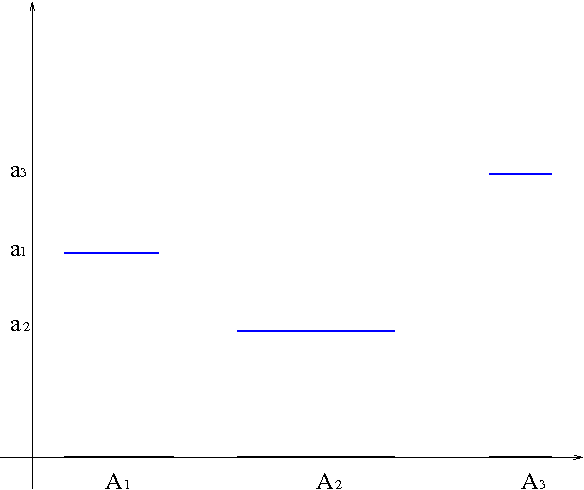
If $A_1,A_2,\cdots,A_m\in\mathscr{U}$ with $\Omega=\bigcup_{i=1}^m A_i$ and $a_1,a_2,\cdots,a_m\in\mathbb{R}$, then
$$X=\sum_{i=1}^m a_iI_{A_i}$$ is a random variable called a simple function.
Lemma. Let $X: \Omega\longrightarrow\mathbb{R}^n$ be a random variable. Then
$$\mathscr{U}(X)=\{X^{-1}(B): B\in\mathscr{B}\}$$ is the smallest $\sigma$-algebra with respect to which $X$ is measurable. $\mathscr{U}(X)$ is called the $\sigma$-algebra generated by $X$.
Definition. A collection $\{X(t)|t\geq 0\}$ of random variables parametrized by time $t$ is called a stochastic process. For each $\omega\in\Omega$, the map $t\longmapsto X(t,\omega)$ is the corresponding sample path.
Let $(\Omega,\mathscr{U},P)$ be a probability space and $X=\sum_{i=1}^k a_iI_{A_i}$ a simple random variable. The probability that $X=a_i$ is $P(X=a_i)=P(X^{-1}(a_i))=P(A_i)$, so $\sum_{i=1}^k a_iP(A_i)$ is the expected value of $X$. We define the integral of $X$ by
\begin{equation}\label{eq:integral}\int_{\Omega}XdP=\sum_{i=1}^k a_iP(A_i)\end{equation}
if $X$ is a simple random variable. A random variable is not necessarily simple so we obviously want to extend the notion of integral to general random variables. First suppose that $X$ is a nonnegative random variable. Then we define
\begin{equation}\label{eq:integral2}\int_{\Omega}XdP=\sup_{Y\leq X,\ Y\ \mbox{simple}}\int_{\Omega}YdP\end{equation}
Let $X$ be a random variable. Let $X^+=\max\{X,0\}$ and $X^-=\max\{-X,0\}$. Then $X=X^+-X^-$. Define
\begin{equation}\label{eq:integral3}\int_{\Omega}XdP=\int_{\Omega}X^+dP-\int_{\Omega}X^-dP\end{equation}For a random variable $X$, we would still call the integral \eqref{eq:integral3} the expected value of $X$ and denote it by $E(X)$. This integral is called Lebesgue integral in real analysis (see [2]). When I first learned Lebesgue integral in my senior year in college, it wasn’t very clear to me as to what motivated one to define Lebesgue integral the way it is. In terms of probability the motivation is so much clear. I personally think that it would be better if we introduce Lebesgue integral to undergraduate students in the context of probability theory rather than abstract real analysis. If $X:\Omega\longrightarrow\mathbb{R}^n$ is a vector-valued random variable and $X=(X_1,X_2,\cdots,X_n)$, we define $$\int_{\Omega}XdP=\left(\int_{\Omega}X_1dP,\int_{\Omega}X_2dP,\cdots,\int_{\Omega}X_ndP\right)$$As one would expect from an integral, the expected value $E(\cdot)$ is linear.
Definition. We call $$V(X)=\int_{\Omega}|X-E(X)|^2dP$$the variance of $X$.
It follows from the linearity of $E(\cdot)$ that $$V(X)=E(|X-E(X)|^2)=E(|X|^2)-|E(X)|^2$$
Lemma. If $X$ is a random variable and $1\leq p<\infty$, then \begin{equation}\label{eq:chebyshev}P(|X|\geq\lambda)\leq\frac{1}{\lambda^p}E(|X|^p)\end{equation}for all $\lambda>0$. The inequality \eqref{eq:chebyshev} is called Chebyshev’s inequality.
Proof. Since $1\leq p<\infty$, $|X|\geq\lambda\Rightarrow |X|^p\geq\lambda^p$. So, \begin{align*}E(|X|^p)&=\int_{\Omega}|X|^pdP\\&\geq\int_{|X|\geq\lambda}|X|^pdP\\
&\geq\lambda^p\int_{|X|\geq\lambda}dP\\&=\lambda^pP(|X|\geq\lambda).\end{align*}
Example. Let a random variable $X$ have the probability density function $$f(x)=\left\{\begin{array}{ccc}\frac{1}{2\sqrt{3}} & \mbox{if} & -\sqrt{3}<x<\sqrt{3}\\ 0 & \mbox{elsewhere}
\end{array}\right.$$For $p=1$ and $\lambda=\frac{3}{2}$, $\frac{1}{\lambda}E(|X|)=\frac{1}{\sqrt{3}}\approx 0.58$. Note that $E(|X|)=\int_{-\infty}^\infty |x|f(x)dx$. (We will discuss this later.) $P(|X|\geq\frac{3}{2})=1-\int_{-\frac{3}{2}}^{\frac{3}{2}}f(x)dx=1-\frac{\sqrt{3}}{2}=0.134$. Hence we confirm Chebyshev’s inequality.
References: Not in particular order
- Lawrence C. Evans, An Introduction to Stochastic Differential Equations, Lecture Notes
- H. L. Royden, Real Analysis, Second Edition, Macmillan
- Robert V. Hogg, Joseph W. McKean, Allen T. Craig, Introduction to Mathematical Statistics, Sixth Edition, Pearson

