In this lecture, we devise a way to calculate the area under a curve. How do we do this? Have you seen the Spaceship Earth at Epcot? If you look at the Spaceship Earth from afar, it looks like a smooth sphere but if you come close, you will find out that it is made of a whole bunch of triangles (actually tetrahedra).

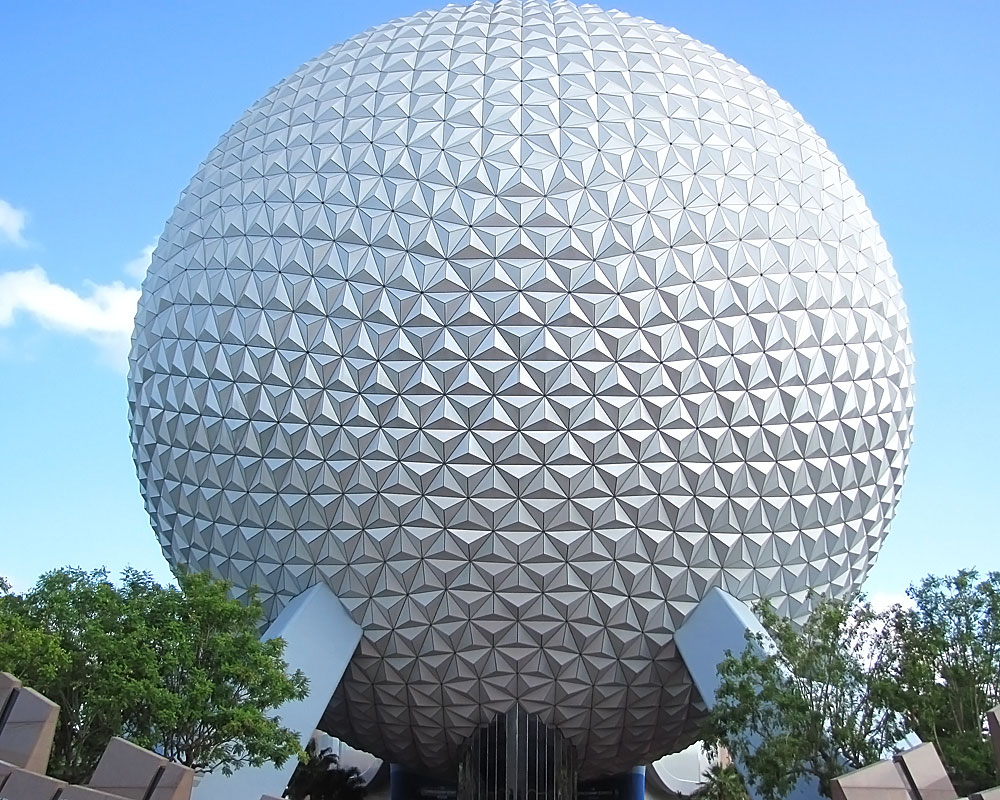
Spaceship Earth

This may give us a clue as to how to tackle our problem. Perhaps we can too to approximate the given curved region with some simple geometric figures of which we know how to calculate areas. Considering that our region is a part of a rectangle except for the curved top, the best candidate would be rectangles. By the way this is in no way a new idea. Ancient Greeks already knew that they could approximate complex curved regions or solids by simple geometric objects such as triangles, rectangles, disks, etc. There are three convenient ways to approximate the area under a curve by rectangles. They are called the left-end point method, midpoint method, and right-end point method, respectively. Let us first discuss the left-end point method. We want to approximate the area under a curve given by $y=f(x)$ on the interval $[a,b]$. Partition $[a,b]$ by $n$ equal subintervals
$$a=x_0<x_1<\cdots<x_n=b,$$
where $\Delta x_k:=\ell([x_{k-1},x_k])=\frac{b-a}{n}$ and $x_k=x_0+k\frac{b-a}{n}$, $k=1,2,\cdots,n$. On each subinterval $[x_{k-1},x_k]$ we consider the rectangle with base $\Delta x_k=\frac{b-a}{n}$ and height $f(x_{k-1})$ (i.e. the left-end point of $[x_{k-1},x_k]$). The area $A$ of the region is then approximated by adding areas of these rectangles:
\begin{align*}
A&\approx f(x_0)\Delta x_1+f(x_1)\Delta x_2+\cdots+f(x_{n-1})\Delta x_n\\
&=\sum_{k=0}^{n-1}f(x_k)\Delta x\\
&=\sum_{k=0}^{n-1}f\left(x_0+k\frac{(b-a)}{n}\right)\frac{b-a}{n}.
\end{align*}
But we are not just satisfied with an approximation. Can we find the exact area $A$? The following figures would give us a clue. The figures show the area under the curve $y=x^2$ on the unit interval $[0,1]$ being approximated by the left-end point method with $n=4$, $n=10$, $n=20$, $n=50$, and $n=100$, respectively.

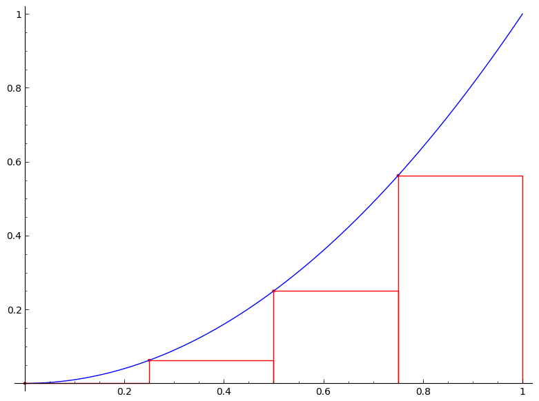
Approximation by the Left-end point method with n=4

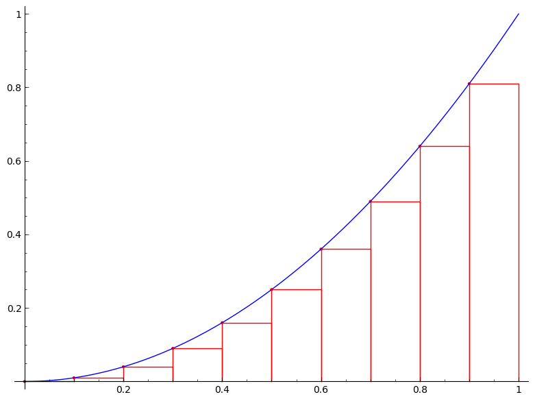
Approximation by the Left-end point method with n=10

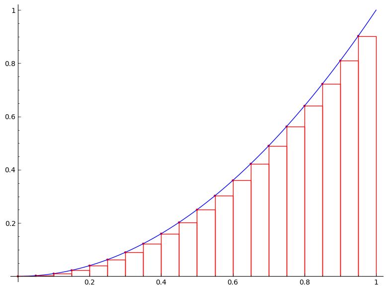
Approximation by the Left-end point method with n=20

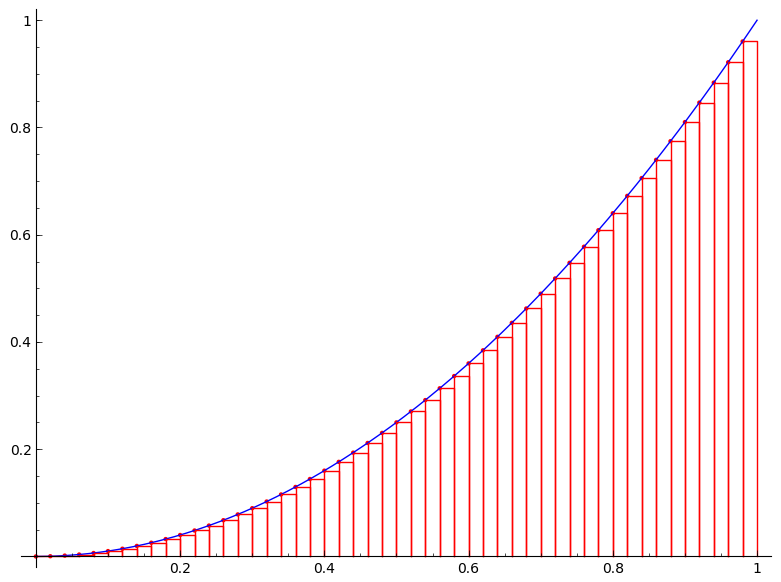
Approximation by the Left-end point method with n=50

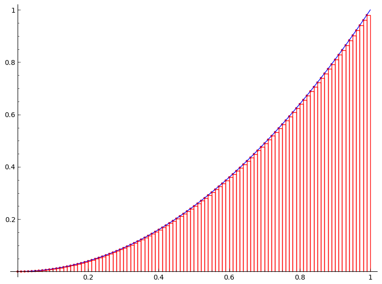
Approximation by the Left-end point method with n=100

It is clear from the above figures that the more rectangles we use the better approximation we get (or equivalently the smaller the error becomes). So if we imagine that we somehow can increase the number of rectangles to infinity, the error will be gone and we will obtain the exact area $A$. How do we then achieve this? Simple, by taking the limit
\begin{equation}\label{eq:left-endpt}
A=\lim_{n\to\infty}\sum_{k=0}^{n-1}f\left(x_0+k\frac{(b-a)}{n}\right)\frac{b-a}{n}.
\end{equation}
Before we discuss an example, let me list three useful sums.
\begin{align}
\label{eq:sum1}
1+2+3+\cdots+n&=\sum_{k=1}^nk=\frac{n(n+1)}{2},\\
\label{eq:sum2}
1^2+2^2+3^3+\cdots+n^2&=\sum_{k=1}^nk^2=\frac{n(n+1)(2n+1)}{6},\\
\label{eq:sum3}
1^3+2^3+3^3+\cdots+n^3&=\sum_{k=1}^nk^3=\left[\frac{n(n+1)}{2}\right]^2.
\end{align}

Example. Let $f(x)=x^2$ and $a=1$, $b=2$. Find the area under the curve $y=f(x)$.

Solution.
\begin{align*}
A&=\lim_{n\to\infty}\sum_{k=0}^{n-1}f\left(1+\frac{k}{n}\right)\frac{1}{n}\\
&=\lim_{n\to\infty}\sum_{k=0}^{n-1}\left(1+\frac{k}{n}\right)^2\frac{1}{n}\\
&=\lim_{n\to\infty}\left\{\frac{1}{n}\sum_{k=0}^{n-1} 1+\frac{2}{n^2}\sum_{k=0}^{n-1}k+\frac{1}{n^3}\sum_{k=0}^{n-1}k^2\right\}\\
&=\lim_{n\to\infty}\left\{\frac{n}{n}+\frac{2}{n^2}\frac{(n-1)n}{2}+\frac{1}{n^3}\frac{(n-1)n(2n-1)}{6}\right\}\\
&=\frac{7}{3}.
\end{align*}

In a similar manner, we can also calculate the area $A$ under curve $y=f(x)$ on the closed interval $[a,b]$ by the midpoint method
\begin{equation}
\label{eq:midpt}
\begin{aligned}
A&=\lim_{n\to\infty}\sum_{k=1}^{n}f\left(\frac{x_{k-1}+x_k}{2}\right)\frac{b-a}{n}\\
&=\lim_{n\to\infty}\sum_{k=1}^{n}f\left(x_0+\frac{(2k-1)}{2}\frac{(b-a)}{n}\right)\frac{b-a}{n},
\end{aligned}
\end{equation}
and by the right-end point method
\begin{equation}\label{eq:right-endpt}
A=\lim_{n\to\infty}\sum_{k=1}^{n}f\left(x_0+k\frac{(b-a)}{n}\right)\frac{b-a}{n}.
\end{equation}

For calculating the exact area under a curve, you can use any of the left-end point, midpoint, and right-end point methods. But what is you are only interested in approximating the area under a curve? Assuming that you are using the same number of rectangles to approximate the area, is there a difference between the methods. If fact, there is. In the above example, we found the exact area $\frac{7}{3}$ of the region under $y=x^2$ on the interval $[1,2].$ The approximation by the left-end point method with $n=100$ is 2.31835. The approximation by the midpoint method with $n=100$ is 2.333325. The approximation by the right-end point method with $n=100$ is 2.34835. Let us now compare the errors from the left-end point, midpoint, and right-end point methods, respectively.
\begin{align*}
E_{\mathrm{left}}&=\left|\frac{7}{3}-2.31835\right|\approx 0.014983333,\\
E_{\mathrm{mid}}&=\left|\frac{7}{3}-2.333325\right|\approx 0.0000083333333,\\
E_{\mathrm{right}}&=\left|\frac{7}{3}-2.34835\right|\approx 0.015016667.
\end{align*}
Clearly, the midpoint method gives rise to the best approximation among the three approximation methods when the same number of rectangles are used. This is indeed true in general. If the function is increasing on the closed interval, the left-end point method underestimates while the right-end point method overestimates. If the functions is decreasing on the closed interval, the left-end point method overestimates while the right-end point method underestimates. The midpoint method averages these two estimates.